Noise-driven Concurrent Stereo Matching

HOME

Location: NCSM >Concurrent Vs. Conventional

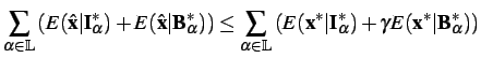
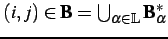
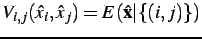
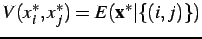
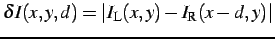
Subsections

Two recent comprehensive overviews provide detailed comparisons of most of the known stereo matching algorithms [4,19]. A stereo test-bed, the Middlebury data set [4], is widely accepted at present as an ad hoc standard for evaluating the accuracy of disparity maps obtained by different algorithms. A number of stereo matching algorithms have been also analysed in a few earlier surveys [20,21,22,23,24,25]. Most stereo algorithms search for the ``best matches'' between areas to be selected as corresponding in the left and right images of a stereo pair. By the matching criteria and optimisation strategy, the algorithms can be placed into two main categories. The first category performs local constrained optimisation in order to individually match relatively small image areas whereas the second category performs global constrained optimisation in order to match entire scan-lines or whole images. This chapter analyses advantages and disadvantages of most popular stereo algorithms, and formulates a new approach to stereo matching which is tested in later chapters.

Stereo Matching by Local Optimisation

These techniques are typically based on maximising cross-correlation between a relatively small window positioned in one image and a like window in another image placed to a set of possible positions. In the simplest case, assuming all the window points have likely the same or very close disparities, the windows in both images have the same fixed size. The correlation allows for contrast and offset deviations between the corresponding image intensities in the windows. However, the constant disparity assumption may not be valid for all the window points. Thus variations of actual disparities and partial occlusions, where one image has areas absent from another, may lead to accumulation of pixel-wise errors which eventually result in false matching. Unstable matching results are obtained on homogeneous image areas with almost constant intensities where correlation peaks reflect only image noise.

Comparing to a more straightforward SSD or the sum of absolute differences (SAD) matching scores, the cross and correlation is effective for taking account of locally uniform contrasr-offset deviations between the corresponding intensities. However, the optimal choices for the window size and shape remain unsolved problems, because the choice depends not only on the known local intensity variations, i.e. the variations in texture, but also on the local variations of the unknown disparities and possible occlusions. Generally, the choice of small windows results in too noisy and unstable correlation values, and larger windows distort an actual disparity pattern. Although the correlation values for large windows are more stable, the search for true disparities becomes less accurate.

To overcome this problem, the window sizes and shapes in both stereo images should vary in accord with expected surface changes. In digital photogrammetry, The least-square correlation [26] was used to synchronously vary window sizes in both the images in accord with an expected slope of a 3D surface. A more recent sophisticated adaptive window matching iteratively varies both the window size and shape in accord with both the local intensity values and current depth estimates [27]. In experiments, such an adaptation improves results of correlation-based stereo matching in smooth and highly textured surface regions. Nonetheless the matching does not account for partial occlusions and therefore tends to smooth surface discontinuities excessively.

Generally, due to accumulation of errors, algorithms based on local optimisation result in very large disparity errors for homogeneous or occluded areas as well as areas with rapidly changing disparity patterns. Also, since only local constraints are used, the reconstructed disparity map may violate physical constraints of surface visibility. Traditionally, such stereo matching is widely used in real-time applications due to its linear time complexity, , where is the number of image pixels and is the window size.

Marr and Poggio provided a simple iterative stereo matching combining local optimisation with global constraints [7]. It takes account of neighbouring matching positions along each pair of corresponding epipolar scanlines in stereo images. For each pair, a 2D interconnected cross-section of the matching score volume in the disparity space is built. Initially, the volume is filled in with the local similarity scores-typically obtained by correlation with small windows. Then the scores are mutually adjusted using excitation and inhibition links between the neighbouring points in the disparity space, the links having enforced the uniqueness and continuity constraints. Weighting factors for the inhibitor links represent the likelihood of pairwise image correspondences. Zitnick and Kanade [28] use instead a fixed 2D excitation region in the same disparity space. Zhang and Kambhamettu [29] take advantage of image segmentation in calculating the initial matching scores using a variable 3D excitation region. The link weights are updated by a simple propagation of the constraints across the neighboring matching points. This iterative adjustment pursues the goal of resolving ambiguities of multiple similar stereo matches. However, because the global constraints are involved to only improve the initialising results, the final accuracy heavily depends on how accurate is the initialisation by local stereo matching.

Stereo Matching by Global Optimisation

The basic drawback of the local techniques is that global constraints imposed by stereo viewing geometry and 3D scene consistency cannot be taken into account directly during the matching process. Due to global uniqueness, continuity and visibility constraints, each ``best match'' restricts other matching possibilities. Typically, an optical surface observed by stereo cameras are described as samples of specific Markov random field (MRF) models such that the constrained local disparity variations are governed by potential functions of neighbouring pairs of disparities or corresponding image signals as well as variations of the corresponding signals under the uniqueness constraint. 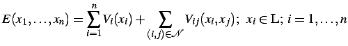Assuming a parallel axis stereo geometry, the matching problem is then formulated as the minimisation of an additive energy function, e.g.

$\begin{displaymath} \begin{array}{l} E(\mathbf{d}\vert\mathbf{g}_1,\mathbf{g}_... ...n}},y+\Delta_{\mathrm{n}^\prime})\right) \right] \end{array} \end{displaymath}$

where

denotes an image-based planar arithmetic lattice supporting both a surface and stereo images represented by the disparity, $\mathbf{d}=[d(x,y): (x,y)\in L]$ , and intensity functions, $\mathbf{g}_1$ and $\mathbf{g}_2$ , respectively, of the lattice coordinates

and

is a point (pixel) neighbourhood in terms of a set of the coordinate increments $(\Delta_\mathrm{n},\Delta_\mathrm{n}^\prime)$ . The like Markovian model can also govern the matching of a homogeneous texture with multiple positions of equally ``best matches'' and take account of partial occlusions where matching of some image areas is in principle impossible. For the most part, such a constrained energy minimisation is quite computationally expensive.

Dynamic Programming

Dynamic programming (DP) is applied to solve a 2D optimisation problem with a goal function by splitting the problem into N 1D optimisation subproblems dealing each with the goal function with the continuity constraints only along the epipolar lines (i.e. with only linear neighbourhoods

). This considerably reduces the computational complexity.

Stereo matching by DP, proposed first by Gimel'farb et al. in 1972 [8] partitions a stereo pair into a set of corresponding epipolar scan-lines and finds the most likely epipolar profile in the disparity space under the linear ordering, uniqueness, and continuity constraints using the Viterbi algorithm. Afterwards, Baker and Binford [9] and independently, many other researchers have developed different stereo matching algorithms exploiting the same or closely similar DP optimisation schemes.

One of the key elements in dynamic programming is how to define pixel-wise signal dissimilarity measure under possible spatially variant contrast-offset distortions of stereo images. The symmetric dynamic programming stereo (SDPS) algorithm introduced by Gimel'farb in 1979 [30] evaluated minimum estimates of most likely contrast and offset intensity distortions during the scanline-to-scanline DP matching. In 1981, Baker and Binford [9] proposed an edge-based DP stereo matching to account implicitly for photometric distortions. The basic idea was to match the corresponding edges of two images of a stereo pair rather than original intensities. Then the disparities for the best edge matches were interpolated over the untextured regions. Unfortunately, such an interpolation cannot preserve sharp discontinuities. Also, the matching itself presumes that the edges are accurately found in both stereo images. A similar DP algorithm is described by Raju, Binford, and Shekar [31].

Later, Ohta and Kanade [32] performed this algorithm with both the intra- and inter-scanline. They treated a path-finding DP problem as a search in a 2D plane where vertical and horizontal axes relate to the right and left scanlines, respectively. A similar algorithm was proposed also by Lloyd [33]. Intille and Bobick [34,35] do not use the continuity constraint at all, relying upon ``ground control points'' to exclude the need for any external smoothness constraint. Geiger, Ladendorf, and Yuille [36] also treat scanlines independently, but suppose that disparities are piecewise constant along each scanline in order to symmetrically enforce strict correspondence between discontinuities and occlusions in stereo images. Cox [37] and Belhumeur and Mumford [38] impose 2D continuity constraints through inter-scanline constraints. Cox [37] counted and minimised the total number of depth discontinuities as a subordinate goal and used either one or two DP stages for efficient approximate minimisation. Belhumeur and Mumford [38] also minimise the number of pixels with discontinuities, but generalise the notion of discontinuity, counting both steps and edges. They introduced a symmetric energy functional incorporating this count and proposed to iteratively minimise it with stochastic DP.

A novel variant of the SDPS [30,39] will be detailed in Chapter as one of the approaches to estimating noise in stereo images. In this algorithm, regularisation with respect to partial occlusions is based on Markov chain models of both epipolar profiles and image intensities along each profile [40]. The algorithm accounts for spatially variant contrast and offset distortions of stereo images by mutual adaptation of the corresponding signals. The adaptation sequentially estimates the ``ground" signals for each binocularly visible point along the profile from the corresponding image signals. The estimated signals are then adapted to each image by changing their increments to within an allowable range.

The principal disadvantage of DP optimisation is that global constraints are applied only along each pair of the epipolar scan-lines; the inter-scanline constraints can be taken into account only approximately, e.g. by iterative alternate matching along and across the scanlines, respectively. The DP algorithms presume a single continuous surface due to the ordering constraint making the corresponding pixels appear in the same order in the left and right scanlines. Obviously, the constraint is not always met. Also, due to intrinsic directionality of DP optimisation, local pixel-wise errors tend to propagate along scanlines, thus corrupting potentially good nearby matches. As a result, the computed disparity maps may display horizontal streaks.

Graph Minimum-cut Optimisation

Unlike the DP matching, graph optimisation techniques use global constraints over the entire 2D images. Matching is formulated as a maximum-flow/minimum-cut problem [41]. Both the stereo images and disparity map are described with a simple Markov random field (MRF) model taking into account the -disparity of and the difference between intensities in each pair of the corresponding points. The contrast and offset distortions are not considered assuming that the compatibility constraint holds. Typically, the MRF model results in the matching score being a 2D sum of data terms measuring the pixel-wise intensity dissimilarities and smoothness terms penalising large surface (disparity) changes over the neighbouring points. Because of multiple disparity values per point, the exact global minimisation of such goal functions is an NP-hard problem, apart from a few special cases with very restrictive conditions on the functions. In principle, the optimisation can be performed with pixel-wise iterative simulated annealing (SA) [42,43]. It makes sequential small stochastic pixel-wise moves in the disparity space that tend to improve the goal function and have a specific ``cooling" schedule to ensure that the random improvement first can reach the global optimum and then stay within a gradually contracting neighbourhood of that optimum. But even in the simplest case of binary labelling [44] where the exact solution can be obtained by the network maximum flow / minimum cut techniques, the SA algorithm converges to a stable point which is too far from the global minimum. Although SA provably converges to the global minimum of energy [42], this could be obtained only in exponential time; this is why no practical implementation can closely approach the optimum [44].

The main drawback of these algorithms is that each iteration changes only one label in a single pixel in accord with the neighboring labels and therefore it results in an extremely small move in the space of possible labelings. Obviously, the convergence rate should become faster under larger moves that simultaneously change labels in a large number of pixels.

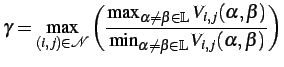
Roy and Cox [45] proposed a much faster approximate method based on the preflow-push lift-to-front optimisation algorithm for finding the maximum flow in a network^2.1. Their method builds an undirected graph for a chosen reference image and finds exactly one disparity for each pixel therein. Ishikawa and Geiger [46] proposed an alternative optimisation method that involves the ordering constraint and furthermore distinguishes between ordinary, edge, and junction pixels. Their method uses a directed graph and symmetrically enforces the uniqueness constraint. Both methods smooth surface discontinuities because functional forms of penalties for discontinuities are heavily restricted (e.g. only the convex energy terms).

Naturally, graph optimisation is computationally complex. Hence, Boykov, Veksler, and Zabih [47] proposed an approximate optimisation technique for a wide variety of non-convex energy terms. Boykov et al [48] subsequently developed a more theoretically justified optimisation technique. It is somewhat less widely applicable, but it produces results provably within a constant factor of the global optimum [49]. Boykov et al. [1] applied these optimisation techniques to stereo matching with the goal energy functions allowing for large $\alpha$ -expansion and $\alpha - \beta$ swap moves in the disparity space. The large moves considerably accelerate the optimisation. Kolmogorov and Zabih [50] proposed more complex graphs for stereo matching. The graph vertices not only represent pixel correspondences but also impose the uniqueness constraints to handle partial occlusions. Their algorithm enforces symmetric two-way uniqueness constraints, but it is limited to constant-disparity continuity.

Large moves using min-cut / max-flow techniques

Two fast approximate algorithms for energy minimization developed by Boykov and Kolmogorov [1] improve the poor convergence of simulated annealing by replacing extremely small pixel-wise moves with large moves involving a large number of pixels simultaneously. The resulting process converges to a solution that in some cases is provably within a known factor of the global energy minimum.

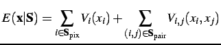
The energy function to be minimized is

$\displaystyle E(x_1,\ldots,x_n) = \sum\limits_{i=1}^n V_i(x_i) + \sum\limits_{(i,j)\in\mathcal{N}}V_{ij}(x_i,x_j);\;\; x_i\in\mathbb{L};\; i=1,\ldots,n$

(2.2.1)

where $\mathbb{L}=\{1,2,\ldots,L\}$ is an arbitrary finite set of labels, $\mathcal{N}\subset\{1,\ldots,n\}^2$ denotes a set of neighboring, or interacting pairs of pixels, $V_i:\mathbb{L}\rightarrow\R$ is a pixel-wise potential function specifying pixel-wise energies in a pixel

under different labels, and $V_{ij}:\mathbb{L}^2\rightarrow\R$ is a pairwise potential function specifying pairwise interaction energies for different labels in a pair

of neighbors. The pixel-wise energies $V_i(\ldots)$ can be arbitrary, but the pairwise interaction energies have to be either semimetric, i.e. satisfy the constraints

$\displaystyle V_{ij}(\alpha,\alpha)=0; \;\; V_{ij}(\alpha,\beta)=V_{ij}(\beta,\alpha)\geq 0\;\; \forall \; \alpha,\beta\in\mathbb{L}$

or metric, i.e. satisfy the same constraints plus the triangle inequality

$\displaystyle V_{ij}(\alpha,\beta)\leq V_{ij}(\alpha,\gamma)+ V_{ij}(\gamma,\beta)\;\; \forall\; \alpha,\beta,\gamma\in\mathbb{L}$

Each pixel labeling, $\mathbf{x}$ , with a finite set of indices $\mathbb{L}=\{1,\ldots,L\}$ partitions the set of pixels, $\mathbf{R}=\{1,\ldots,n\}$ , into

disjoint subsets, $\mathbf{R}_\lambda=\{i\vert i\in\mathbf{R};\;x_i=\lambda\in\mathbb{L}\}$ (some of them may be empty), i.e. creates a partition $\mathbf{P} =\{\mathbf{R}_\lambda : \lambda=1,\ldots,L\}$ . Each change of a labeling, $\mathbf{x}$ , changes the corresponding partition, $\mathbf{P}$ .

The approximate Boykov-Veksler-Zabih minimization algorithms work with any semimetric or metric, $V_{ij}$ , by using large $\alpha$ - $\beta$ -swap or $\alpha$ -expansion moves respectively. The conditionally optimal moves are found with a min-cut / max-flow technique.

The $\alpha$ - $\beta$ -swap

for an arbitrary pair of labels, $\alpha\beta\in\mathbb{L}$ , is a move from a partition, $\mathbf{P}$ , for a current labeling, $\mathbf{x}$ , to a new partition, $\mathbf{P}^\prime$ , for a new labeling, $\mathbf{x}^\prime$ , such that $\mathbf{R}_\lambda = \mathbf{R}^\prime_\lambda$ for any label, $\lambda \ne \alpha, \beta$ . In other words, this move changes only the labels $\alpha$ and $\beta$ in their current region, $\mathbf{R}_{\alpha\beta}=\mathbf{R}_\alpha\cup\mathbf{R}_\beta$ , whereas all the other labels in $\mathbf{R}\backslash\mathbf{R}_{\alpha\beta}$ remain fixed. In the general case, after the $\alpha$ - $\beta$ -swap, some pixels change their labels from $\alpha$ to $\beta$ and some others from $\beta$ to $\alpha$ . A special variant is when the label $\alpha$ is assigned to some pixels previously labeled $\beta$ .

The $\alpha$ -expansion

of an arbitrary label, $\alpha$ , is a move from a partition, $\mathbf{P}$ , for a current labeling, $\mathbf{x}$ , to a new partition, $\mathbf{P}^\prime$ , for a new labeling, $\mathbf{x}^\prime$ , such that $\mathbf{R}_\alpha \subset \mathbf{R}^\prime_\alpha$ and $\mathbf{R}\backslash\mathbf{R}_\alpha^\prime= \cup_{\lambda\in\mathbb{L};\;\l... ...ash\mathbf{R}_\alpha= \cup_{\lambda\in\mathbb{L};\;\lambda\ne\alpha}\mathbf{R}$ . In other words, after this move, any subset of pixels can change their labels to $\alpha$ .

Energy minimization algorithms

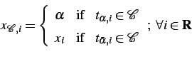
The SA and ICM algorithms apply pixel by pixel relaxation moves changing one label each time. These moves are both $\alpha$ - $\beta$ -swap and $\alpha$ -expansion, so that they generalize the standard relaxation scheme. The algorithms based on these generalizations are sketched in Fig.

**Figure:** $\sf$ Block-diagrams of the approximate minimization algorithms proposed in [1].
$% latex2html id marker 2766 \fbox{ \begin{minipage}{140mm} \centerline{~\\ \t... ...d output the final labeling $\mathbf{x}$ \end{description} \end{minipage} }$

An iteration at Step 2 performs individual $\alpha$ -expansion moves in the expansion algorithm and individual $\alpha$ - $\beta$ -swap moves in the swap algorithm. It is possible to prove that the minimization terminates in a finite number of iterations being of order of the image size . Actually, image segmentation and stereo reconstruction experiments [51,1] have shown that these algorithms converge to the local energy minimum just in a few iterations.

Given a current labeling $\mathbf{x}$ (partition $\mathbf{P}$ ) and a pair of labels $(\alpha,\beta)$ or a label $\alpha$ , the swap or expansion move, respectively, at Step 2.1 in Fig. uses the min-cut / max-flow optimization techique to find a better labeling, $\hat{\mathbf{x}}$ . The latter minimizes the energy over all labelings within one $\alpha$ - $\beta$ -swap (the swap algorithm) or one $\alpha$ -expansion (the expansion algorithm) of $\mathbf{x}$ and corresponds to a minimum cut of a specific graph. The swap and expansion graphs are different, and the exact number of their pixels, their topology and the edge weights vary from step to step in accord with the current partition.

Swap algorithm: finding the optimal move

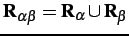
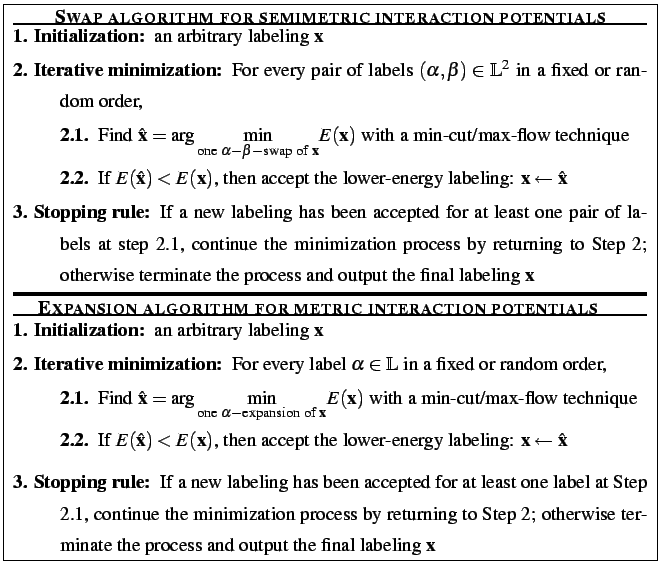
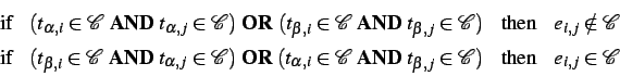
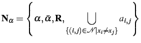
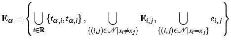
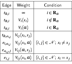
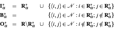
The graph, $\mathbf{G}_{\alpha\beta} = [\mathbf{N}_{\alpha\beta};\mathbf{E}_{\alpha\beta}]$ , in Fig. for finding an optimal swap-move is built only on the pixels, $i\in\mathbf{R}_{\alpha\beta}=\mathbf{R}_\alpha\cup\mathbf{R}_\beta$ , having labels, $\alpha$ and $\beta$ , in the partition, $\mathbf{P}$ , corresponding to the current labeling, $\mathbf{x}$ . The set of nodes, $\mathbf{N}_{\alpha\beta}$ , includes the two terminals, denoted $\alpha$ and $\beta$ , and all the pixels in $\mathbf{R}_{\alpha\beta}$ . Each pixel, $i\in\mathbf{R}_{\alpha\beta}$ , is connected to the terminals, $\alpha$ and $\beta$ , by edges $t_{\alpha,i}$ and $t_{\beta,i}$ -called -links (terminal links) [1]. Each pair of nodes, $(i,j)\subset\mathbf{R}_{\alpha\beta}$ , which are neighbors, i.e. $(i,j)\in\mathbf{E}$ , is connected with an edge, $e_{i,j}$ , called an -link (neighbor link) [1]. Therefore, the set of edges, $\mathbf{E}_{\alpha\beta}$ , consists of the - and -links.

**Figure:** $\sf$ Example graph, $( \mathbf{G}_{ \alpha\beta })$ , for finding the optimal swap move for the set of pixels, $\mathbf{R}_{\alpha\beta}=\mathbf{R}_\alpha\cup\mathbf{R}_\beta$ , with the labels, $\alpha$ and $\beta$ .
$\includegraphics[width=90mm]{ab-swap.eps}$

If the edges have the following weights:

$\begin{displaymath} \begin{array}{\vert c\vert c\vert c\vert}\hline \mathsf{Ed... ...hcal{N}\cap\mathbf{R}_{\alpha\beta}^2 \\ \hline \end{array} \end{displaymath}$

then each cut $\mathcal{C}$ on $\mathbf{G}_{\alpha\beta}$ must include exactly one

-link for any pixel, $i\in\mathbf{R}_{\alpha\beta}$ : otherwise, either there will be a path between the terminals if both the links are included, or a proper subset of $\mathcal{C}$ will become a cut if both the links are excluded. Therefore, any cut, $\mathcal{C}$ , provides a natural labeling, $\mathbf{x}_{\mathcal{C}}$ , such that every pixel, $i\in\mathbf{R}_{\alpha\beta}$ is labeled with $\alpha$ or $\beta$ if the cut $\mathcal{C}$ separates

from the terminal $\alpha$ or $\beta$ , respectively, and the other pixels keep their initial labels (Fig.

$\begin{displaymath} x_{\mathcal{C},i} = \left\{ \begin{array}{lll} \alpha & \... ...{\alpha\beta} \end{array} \right.;\; \forall i\in\mathbf{R} \end{displaymath}$

Each labeling $\mathbf{x}_\mathcal{C}$ corresponding to a cut, $\mathcal{C}$ , on the graph $\mathbf{G}_{\alpha\beta}$ is one $\alpha$ - $\beta$ -swap away from the initial labeling, $\mathbf{x}$ .

**Figure:** $\sf$ A cut, $\mathcal{C}$ , on $\mathbf{G}_{\alpha\beta}$ for two pixels, $i,j\in\mathcal{N}$ , connected by an -link $(e_{i,j})$ : dashed edges are cut by $(\mathcal{C}$ .
$\includegraphics[width=90mm]{ab-cuts.eps}$

Because a cut separates a subset of pixels in $\mathbf{R}_{\alpha\beta}$ associated with one terminal from a complementary subset of pixels associated with another terminal, it includes (i.e. severs in the graph) an -link, $e_{i,j}$ , between the neighboring pixels in $\mathbf{R}_{\alpha\beta}$ if and only if the pixels and are connected to different terminals under this cut:

$\begin{displaymath} \begin{array}{llll} \mathrm{if}& (t_{\alpha,i}\in\mathcal{... ...al{C}) & \mathrm{then} & e_{i,j}\in\mathcal{C} \end{array} \end{displaymath}$

By taking into account that $V_{ij}(x_{\mathcal{C},i},x_{\mathcal{C},j})$ is a semimetric and by considering possible cuts involving

-links of and

-link between

and

and the corresponding labelings, it is possible to prove:

THEOREM 2.1 (Boykov, Veksler, Zabih, 2001 [1]) There is an one-to-one correspondence between cuts, $\mathcal{C}$ , on $\mathbf{G}_{\alpha\beta}$ and labelings, $\mathbf{x}_\mathcal{C}$ , that are one $\alpha$ - $\beta$ swap from $\mathbf{x}$ . The capacity of a cut $\mathcal{C}$ on $\mathbf{G}_{\alpha\beta}$ is $c(\mathcal{C})=E(\mathbf{x}_\mathcal{C})$ plus a constant where $E(\ldots)$ is the energy of Eq. ().

COROLLARY 2.1 (Boykov, Veksler, Zabih, 2001 [1]) The lowest energy labeling within a single $\alpha$ - $\beta$ -swap move from a current labeling, $\mathbf{x}$ , is the labeling, $\hat{\mathbf{x}}=\mathbf{x}_{\mathcal{C}^\circ}$ , corresponding to the minimum cut, $\mathcal{C}^\circ$ , on $\mathbf{G}_{\alpha\beta}$ .

Expansion algorithm: finding the optimal move

The set of nodes, $\mathbf{N}_{\alpha}$ , of the graph, $\mathbf{G}_{\alpha} = [\mathbf{N}_{\alpha};\mathbf{E}_{\alpha}]$ , for finding an optimal expansion-move (see a simple 1D example in Fig. ) includes the two terminals, denoted $\alpha$ and $\bar{\alpha}$ , all the pixels, $i\in\mathbf{R}$ , and a set of auxiliary nodes for each pair of the neighboring nodes, $(i,j)\in\mathcal{N}$ , that have different labels $x_i\ne x_j$ in the current partition, $\mathbf{P}$ . The auxiliary nodes are on the boundaries between sets in the partition, $\mathbf{R}_\lambda$ ; $\lambda\in\mathbb{L}$ . Thus the set of nodes is

$\displaystyle \mathbf{N}_\alpha =\left\{ \alpha,\bar{\alpha},\mathbf{R}, \bigcup\limits_{ \{ (i,j)\in\mathcal{N} \vert x_i\ne x_j \}}a_{i,j} \right\}$

**Figure:** $\sf$ Example graph, $\mathbf{G}_{ \alpha }$ , for finding the optimal expansion move for the set of pixels in the image. Here, the set of pixels is $\mathbf{R}=\{i,j,k,l,m\}$ , and the current partition is $\mathbf{P}=\{\mathbf{R}_\alpha$ , $\mathbf{R}_\beta,\mathbf{R}_\gamma\}$ where $\mathbf{R}_\alpha=\{i\}$ , $\mathbf{R}_\beta=\{j,k\}$ , and $\mathbf{R}_\gamma =\{l,m\}$ . Two auxiliary nodes, $a_{i,j}$ and $a_{k,l}$ , are added between the neighboring pixels with different labels in the current partition, i.e. at the boundaries of the subsets, $\mathbf{R}_\lambda$ .
$\includegraphics[width=90mm]{a-expan.eps}$

Each pixel, $i\in\mathbf{R}$ , is connected to the terminals, $\alpha$ and $\bar{\alpha}$ by -links $t_{\alpha,i}$ and $t_{\bar{\alpha},i}$ , respectively. Each pair of neighboring nodes, $(i,j)\subset\mathcal{N}$ , that are not separated in the current partition, i.e. have the same labels in the current labeling, is connected with an -link $e_{i,j}$ . For each pair of the separated neighboring pixels, $(i,j)\in\mathcal{N}$ , that $x_i\ne x_j$ , the introduced auxiliary node, $a_{i,j}$ , results in three edges, $\mathbf{E}_{i,j}=\{e_{i,a_{i,j}},e_{a_{i,j},j},t_{ \bar{\alpha}, a_{i,j} } \}$ , where the first pair of -links connects the pixels and to the auxiliary node $a_{i,j}$ , and the -link connects the auxiliary node, $a_{i,j}$ , to the terminal, $\bar{\alpha}$ . Therefore, the set of all edges, $\mathbf{E}_{\alpha}$ , is

$\displaystyle \mathbf{E}_\alpha =\left\{ \bigcup\limits_{i\in\mathbf{R}}\left\... ..., \bigcup\limits_{ \{(i,j)\in\mathcal{N}\vert x_i = x_j\} }e_{i,j} \right\}$

The edges have the following weights:

$\begin{displaymath} \begin{array}{\vert c\vert c\vert c\vert}\hline \mathsf{Ed... ...ha) & (i,j)\in\mathcal{N};\;x_i = x_j \\ \hline \end{array} \end{displaymath}$

That any cut, $\mathcal{C}$ , on $\mathbf{G}_{ \alpha }$ must include exactly one

-link for any pixel, $i\in\mathbf{R}$ , provides a natural labeling, $\mathbf{x}_{\mathcal{C}}$ , corresponding to the cut (Fig.

$\begin{displaymath} x_{\mathcal{C},i} = \left\{ \begin{array}{lll} \alpha & \... ...in\mathcal{C} \end{array} \right.;\; \forall i\in\mathbf{R} \end{displaymath}$

Each labeling, $\mathbf{x}_\mathcal{C}$ , corresponding to a cut, $\mathcal{C}$ , on the graph, $\mathbf{G}_{ \alpha }$ , is one $\alpha$ -expansion away from the initial labeling $\mathbf{x}$ .

**Figure:** $\sf$ A minimum cut $(\mathcal{C})$ on $( \mathbf{G}_{ \alpha\beta })$ for two pixels $(i,j\in\mathcal{N})$ such that $(x_i\ne x_j)$ ( $(a \equiv a_{i,j})$ is an auxiliary node between the neighboring pixels and ; dashed edges are cut by $(\mathcal{C})$ .
$\includegraphics[width=90mm]{aex-cuts.eps}$

Because a cut separates a subset of pixels in $\mathbf{R}$ associated with one terminal from a complementary subset of pixels associated with another terminal, it severs an -link, $e_{i,j}$ , between the neighboring pixels, $(i,j)\in\mathcal{N}$ , if and only if the pixels and are connected to different terminals under this cut. Formally:

$\begin{displaymath}\begin{array}{llllll} \mathrm{if} & t_{\alpha,i},t_{\alpha,j... ...athcal{C} & \mathrm{then} & e_{i,j}\in\mathcal{C} \end{array}\end{displaymath}$

(2.2.2)

The triplet of edges, $\mathbf{E}_{i,j}$ , corresponding to a pair of neighboring pixels, $(i,j)\in\mathcal{N}$ , that $x_i\ne x_j$ may be cut in different ways, even when the pair of severed

-links at

and

are fixed. However, a minimum cut uniquely defines the edges to sever in $\mathbf{E}_{i,j}$ in these cases due to the minimality of the cut and the metric properties of the potentials associated with the edges, $\{e_{i,a_{i,j}},e_{a_{i,j},j},t_{\bar{\alpha},a_{i,j}}\}\in\mathbf{E}_{i,j}$ . The triangle inequality suggests that it is always better to cut any one of them, rather than the other two together. This property of a minimum cut, $\mathcal{C}$ , is illustrated in Fig.

and has the following formal representation: if $(i,j)\in\mathcal{C}$ and $x_i\ne x_j$ , then $\mathcal{C}$ satisfies the conditions

$\begin{displaymath}\begin{array}{llll} \mathrm{if} & t_{\alpha,i},t_{\alpha,j}\... ... & \mathcal{C}\cup\mathbf{E}_{i,j} = e_{a_{i,j},j} \end{array}\end{displaymath}$

(2.2.3)

These properties may hold for non-minimal cuts, too. If an elementary cut is defined as a cut satisfying the conditions in Eqs. (

) and (

), then it is possible to prove

THEOREM 2.2 (Boykov, Veksler, Zabih, 2001 [1]) Let a graph, $\mathbf{G}_{ \alpha }$ , be constructed given a labeling $\mathbf{x}$ and $\alpha$ . Then, there is an one-to-one correspondence between elementary cuts on $\mathbf{G}_{ \alpha }$ and labelings within one $\alpha$ -expansion from $\mathbf{x}$ . The capacity of any elementary cut $\mathcal{C}$ is $c(\mathcal{C})=E(\mathbf{x}_\mathcal{C})$ where $E(\ldots)$ is the energy of Eq. .

COROLLARY 2.2 (Boykov, Veksler, Zabih, 2001 [1]) The lowest energy labeling within a single $\alpha$ -expansion move from $\mathbf{x}$ is the labeling, $\hat{\mathbf{x}}=\mathbf{x}_{\mathcal{C}^\circ}$ , corresponding to the minimum cut, $\mathcal{C}^\circ$ , on $\mathbf{G}_{ \alpha }$ .

Optimality of large moves

Although the swap move algorithm has a wider application, as it has only semimetric requirements on potentials $V_{i,j}(\ldots)$ , generally it possesses no proven optimality properties. However, a local minimum obtained with the expansion move algorithm is within a fixed factor of the global minimum, according to

THEOREM 2.3 (Boykov, Veksler, Zabih, 2001 [1]) Let $\hat{\mathbf{x}}$ be a labeling for a local energy minimum when with the expansion moves are allowed, and let $\mathbf{x}^\ast$ be the globally optimal solution. Then, $E( \hat{\mathbf{x} } ) \leq 2 \gamma E ( \mathbf{x}^\ast )$ where

$\displaystyle \gamma = \max\limits_{(i,j)\in\mathcal{N}} \left( \frac{ \max_{\... ...beta) } { \min_{\alpha\ne\beta\in\mathbb{L}}V_{i,j}(\alpha,\beta) } \right)$

Proof. Let some $\alpha\in\mathbb{L}$ be fixed and let $\mathbf{R}_\alpha^\ast =\left\{i\in\mathbf{R}\vert\mathbf{x}^\ast_i=\alpha\right\}$ . Let $\mathbf{x}_\alpha$ be a labeling within one $\alpha$ -expansion move from $\hat{\mathbf{x}}$ such that

$\begin{displaymath} x_{\alpha,i} = \left\{ \begin{array}{lll} \alpha & \mathr... ... \multicolumn{2}{l}{\mathrm{otherwise}} \end{array} \right. \end{displaymath}$

Since $\hat{\mathbf{x}}$ is a local minimum if expansion moves are allowed,

$\displaystyle E(\hat{\mathbf{x}}) \leq E(\mathbf{x}_\alpha)$

(2.2.4)

Let $\mathbf{S} = \mathbf{S}_\mathrm{pix}\cup\mathbf{S}_\mathrm{pair}$ be union of an arbitrary subset, $\mathbf{S}_\mathrm{pix}$ , of pixels in $\mathbf{R}$ ; $\mathbf{S}_\mathrm{pix}\subseteq\mathbf{R}$ , and of an arbitrary subset, $\mathbf{S}_\mathrm{pair}$ , of neighboring pixels in $\mathcal{N}$ ; $\mathbf{S}_\mathrm{pair}\subseteq\mathcal{N}$ . A restriction of the energy of labeling $\mathbf{x}$ to $\mathbf{S}$ is defined as

$\displaystyle E(\mathbf{x}\vert\mathbf{S}) = \sum\limits_{i\in\mathbf{S}_\mathrm{pix}}V_i(x_i)+ \sum\limits_{(i,j)\in\mathbf{S}_\mathrm{pair}}V_{i,j}(x_i,x_j)$

Let $\mathbf{I}_\alpha$ , $\mathbf{B}_\alpha$ , and $\mathbf{O}_\alpha$ denote the union of pixels and pairs of neighboring pixels contained inside, on the boundary and outside of $\mathbf{R}_\alpha^\ast$ , respectively:

$\begin{displaymath} \begin{array}{lllll} \mathbf{I}_\alpha^\ast & = & \mathbf{... ...a^\ast; j\notin\mathbf{R}_\alpha^\ast\right \} \end{array} \end{displaymath}$

The following three relationships hold:

$\displaystyle \mathsf{(a):}\, E(\mathbf{x}_\alpha\vert\mathbf{I}_\alpha^\ast) =... ...ert\mathbf{O}_\alpha^\ast) = E(\hat{\mathbf{x}} \vert\mathbf{O}_\alpha^\ast)$

The relationships (a) and (c) follow directly from the definitions of $\mathbf{R}^\ast_\alpha$ and $\mathbf{x}_\alpha$ . The relationship (b) holds because $V_{i,j}(x_{\alpha,i},x_{\alpha,j})\leq \gamma V(x_i^\ast,y_i^\ast)\ne 0$ for any $(i,j)\in\mathbf{B}_\alpha^\ast$ .

The union $\mathbf{I}_\alpha^\ast \cup \mathbf{B}_\alpha^\ast \cup \mathbf{O}_\alpha^\ast$ includes all the pixels in $\mathbf{R}$ and all the neighboring pairs of pixels in $\mathcal{N}$ . Therefore, Eq. () can be rewritten as

$\displaystyle E(\hat{\mathbf{x}}\vert\mathbf{I}_\alpha^\ast) + E(\hat{\mathbf{... ...ert\mathbf{B}_\alpha^\ast) + E(\mathbf{x}_\alpha\vert\mathbf{O}_\alpha^\ast)$

By substituting the relationships (a)-(c), one can obtain:

$\displaystyle E(\hat{\mathbf{x}}\vert\mathbf{I}_\alpha^\ast) + E(\hat{\mathbf{... ...\mathbf{I}_\alpha^\ast) + \gamma E(\mathbf{x}^\ast\vert\mathbf{B}_\alpha^\ast)$

(2.2.5)

To get the bound on the total energy, Eq. (

) has to be summed over all the labels $\alpha\in\mathbb{L}$ :

$\displaystyle \sum\limits_{\alpha\in\mathbb{L}}\left( E(\hat{\mathbf{x}}\vert\... ...{I}_\alpha^\ast) + \gamma E(\mathbf{x}^\ast\vert\mathbf{B}_\alpha^\ast)\right)$

(2.2.6)

For every $(i,j)\in\mathbf{B}=\bigcup_{\alpha\in\mathbb{L}}\mathbf{B}_\alpha^\ast$ , the term $V_{i,j}(\hat{x}_i,\hat{x}_j)=E(\hat{\mathbf{x}}\vert\{(i,j)\})$ appears twice on the left side of Eq. (

): once in $E(\hat{\mathbf{x}}\vert\mathbf{B}_\alpha^\ast)$ for $\alpha = x^\ast_i$ , and once in $E(\hat{\mathbf{x}}\vert\mathbf{B}_\alpha^\ast)$ for $\alpha=x^\ast_j$ . Similarly, every $V(x^\ast_i,x^\ast_j)=E(\mathbf{x}^\ast\vert\{(i,j)\})$ appears $2\gamma$ times on the right side of Eq. (

). Therefore, Eq. (

) can be rewritten as

$\displaystyle E(\hat{\mathbf{x}})+E(\hat{\mathbf{x}}\vert\mathbf{B}) \leq E(\m... ...(2\gamma -1)E(\mathbf{x}^\ast\vert\mathbf{B}) \leq 2\gamma E(\mathbf{x}^\ast)$

to give the bound of $2\gamma$ for the factor of the global minimum. $\qedsymbol$

Belief Propagation (BP) Optimisation on Graphs

Unlike the minimum-cut algorithms that find an approximate minimum of an energy function, belief propagation (BP) techniques pass messages and update belief values over the Markovian belief network in order to find an optimum labelling. The message from a node consists of its label (i.e. the disparity value) and the confidence about the state of the node. This confidence can be efficiently computed with the truncated linear model [52]. The messaging illustrated in Figure can be considered as an iterative action in which each node receives messages from its neighbours and then a new belief about each node is computed. Global constraints govern the propagation of information from each stable matching point to neighbouring unstable and likely occluded ones until the propagation process converges. In most cases, colour segments of a reference image constrain confidence propagation to each region.

**Figure:** Local message passing in a graph with six neighbors X1, X2, X3, X4, Y1 and Y2
$\includegraphics[width=2.2in]{bp.eps}$

**Figure:** $\sf$ The Belief Propagation algorithm.
$% latex2html id marker 2854 \fbox{ \begin{minipage}{140mm} \centerline{~\\ \t... ...ing a stable energy value. \end{description} \vspace*{-3mm} \end{minipage} }$

Figure summaries BP algorithm. Many BP implementations [52,53,54,55,56] perform iterative global optimisation using the max-product BP algorithm. In experiments with the Middlebury stereo test-bed [4], these optimisation techniques achieved the highest ranking .

Other global optimisation techniques

Apart from the powerful graph-cut algorithms, other approximate techniques have been used for stereo matching by global energy minimisation. In particular, Saito and Mori [57] in 1995 first applied a genetic algorithm (GA) to stereo vision. Different window sizes were used to find several candidate disparity values at each pixel location, and then the GA selected the disparity for each pixel from these candidates under the global continuity and uniqueness constraints and the assumption that the correct disparity must be among the candidates found. Gong and Yang extended this algorithm by considering both occlusions and false matches [58]. The improved algorithm could detect and remove occlusions and mismatches that violate the visibility constraints.

Layered Algorithms

Layered models provide a new avenue for stereo matching. They allow separate patches at different positions in a 3D scene rather than only a single surface and reconstruction of piecewise smooth surfaces. The primary advantage of this model is that each pixel being the minimum element in the previous methods can be placed semantically to image regions and each surface patch for the image region can get its own identification. Hence, it is possible to model hidden connections among visible surface patches or isolate occluding regions.

Modelling of surface layers helps to avoid many incorrect decisions stemming from the ``best matching" by the signal correspondence. When combining layers, there need not be exactly one surface per pixel. Instead, the pixel correspondences are grouped into candidate volumes or labelled with no surface for an occluded region. By warping a reference left image according to an initial depth map, Baker, Szeliski, and Anandan [59] developed a layered method for stereo matching that minimises the re-synthesis error between the warped right image and the real right view. The disparity of each surface patch is modelled as a plane with small local variations that is similar to the model for a window correlation. The surface continuity is enforced by spatial smoothing of the matching likelihood scores.

Considering connected or slant surfaces, Birchfeld and Tomasi [60] assigned pixels to surfaces using the graph-based techniques of Boykov-Veksler-Zabih [47]. Boundaries along the intensity edges were constrained by assigning exactly one disparity value for each image location. Lin and Tomasi [61] extended this work using the most significant symmetric differences between the input images and a spline model for the layers. Tao and Sawhney [62,63] described a colour segment-based stereo framework for a layered model. They assume small disparity discontinuities inside homogeneous color segments if a disparity hypothesis is correct. As Baker et al. [59], they also warp a reference image to another view in line with an initial depth map and render the image to match the real scene. Then, the minimisation of the global image similarity energy leads the final result. Segmentation reduces the dimensions of disparity space and ensures the disparity smoothness over homogeneous regions. The expensive warping and inference of reasonable disparities for unmatched regions can be avoided with a greedy local search based on a neighbouring disparity hypothesis. Bleyer and Gelautz [64] extended this framework and applied a modified mean-shift algorithm [65,66] embedding planar dissimilarity measurements to extract clusters of similar disparity segments. Hence, the algorithm has the same limitation, namely, the input images have to be well approximated by a set of planes. In other words, the segmentation must accurately find real layers existing in an observed scene. Generally, this cannot be guaranteed if the scene contains objects with more complex surface structures.

A New Proposal: Concurrent Stereo Matching

Drawbacks of Conventional Algorithms

The preceding brief overview highlights what are the main disadvantages of published algorithms. Almost all conventional stereo approaches other than the layered algorithms, search for a single optical surface that yields the best correspondence between the stereo images under constrained surface continuity, smoothness, and visibility. Most of the constraints are ``soft", i.e. limited deviations are allowed. The matching scores used are ad hoc linear combinations of individual terms measuring signal similarity, surface smoothness, surface visibility and occlusions with empirically chosen weights for each term.

The resulting NP-hard global optimisation problem is approximately solved with many different techniques, e.g. dynamic programming [39,67,32,68], belief propagation [53,54] or graph min-cut algorithms [37,1,69]. However, the chosen values of the weights in the matching score strongly influence the reconstruction accuracy [11]. In addition, most of the conventional matching scores take no account of spatially constant or variant contrast and offset deviations. Typical stereo pairs contain many admissible matches, so that the ``best" matching may lead to many incorrect decisions. Moreover, real scenes very rarely consist of a single surface, so this assumption is also too restrictive.

Figure illustrates problems that can be encountered with single surface binocular stereo reconstruction as well as with regularisation of stereo matching for a multiple surface scene. A section through a set of surfaces along with the corresponding piecewise-constant intensity profiles in the left and right images is shown in Figure (a). Grey areas in Figures (b)-(d) show matching regions. Figure (b) shows that an erroneous single surface profile may easily be constructed by applying smoothness and ordering constraints. Other reconstructions (from the many possible) are shown in Figures (c) and (d). Moreover, the corresponding (precisely matching) areas do not reflect the actual scene unless occlusions are taken into account. Without additional constraints, it is impossible to discriminate between possible solutions.

Figure: Multiple and single profile reconstructions from a stereo pair with piecewise-constant signals for corresponding regions: (a) actual disjoint surface profiles; (b) signal-based corresponding areas within a single continuous profile, (c) one (extreme) disjoint variant, and (d) one restricted to a fixed disparity range.

$\includegraphics[width=6cm]{new_st0}$	$\includegraphics[width=6cm]{st-singlet}$
(a)	(b)
$\includegraphics[width=6cm]{st-multip}$	$\includegraphics[width=6cm]{st-multip-range-gs}$
(c)	(d)

Furthermore, even low level signal noise that does not mask major signal changes in Fig. hinders the conventional matching paradigm because it is based on the maximum similarity between the signals for a reasonably constrained surface. In this simple example, the closest similarity between the initially equal signals distorted with independent noise can lead to selection of a completely random surface from a set of admissible variants specified by both signal correspondences and surface constraints.

Given a noise model, a more realistic stereo matching goal is to estimate signal noise and specify a plausible range of differences between corresponding signals. The noise estimates allow us to outline 3D volumes that contain all the surfaces ensuring a `good matching'. Then the desired surface or surfaces may be chosen using surface constraints only.

Figure: `Tsukuba' stereo pair: distribution of signal differences (top left), $\delta I$ , and grey-coded absolute signal differences (bottom right), $\vert \delta I\vert$ , for one pair of epipolar lines (y=173) vs. the actual profile.

$\includegraphics[width=4.32cm,height=4.32cm]{new_newnoisedistrub}$	$\includegraphics[width=5.81cm]{tsukuba-r-173marked}$
$\includegraphics[width=4.32cm]{tsukuba-l-173marked_rot90}$	$\includegraphics[width=5.81cm]{color-173-err-cnt}$

Generally, stereo matching presumes the availability of a signal similarity model that accounts for changes in surface reflection for any potential noise sources. However, most stereo matching scores in computer vision, including the best-performing graph minimum-cut or belief propagation ones, use very simple intensity dissimilarity terms such as the sum of absolute signal differences (SAD) or square differences (SSD) for all the binocularly visible surface points. The underlying signal model assumes equal corresponding signals distorted by an additive independent noise with the same zero-centred symmetric probability distribution. Such a simplification is justified for a few stereo pairs typically used for testing algorithms in today's computer vision, e.g., for the Middlebury data set [4]. However, this simplification is totally invalid in most practical applications, e.g. for aerial or ground stereo images of terrain collected at different times under changing illumination and image acquisition conditions. More realistic similarity models must take account of global or local offset and contrast signal distortions [67,68].

**Table 2.1:** Distribution of intensity differences for corresponding points in the `Tsukuba' scene: % of the corresponding points with the absolute intensity difference $\delta I$ in the indicated range where x-disparities are derived from the ground truth (True) and the model reconstructed by SDPS, GMC and BP algorithms. The final column contains D, the sum of square distances between the distributions for the ground truth and the reconstructed models.
$\delta I$	0	1	2	3- 5	6- 10	11- 20	21- 30	31- 60	61- 125	126- 255	D $\times 10^{-4}$
True	18.5	29.6	19.5	19.1	6.6	3.7	1.4	1.2	0.4	0.0
SDPS	20.9	30.9	18.1	17.9	6.7	3.7	1.2	0.6	0.0	0.0	8.5
GMC	17.2	25.3	15.5	17.3	8.9	6.9	3.3	2.2	1.4	0.0	60.9
BP	17.2	30.4	19.7	21.5	6.4	3.6	1.0	0.8	2.3	1.2	13.6

For the `Tsukuba' stereo pair from the Middlebury data set [4], Table

shows empirical probability distributions of absolute pixel-wise signal differences, $\delta I(x,y,d) = \vert I_\mathrm{L}(x,y) - I_\mathrm{R}(x-d,y) \vert$ , for the corresponding points in the supplied "ground truth" and for three single-surface models reconstructed by symmetric dynamic programming stereo (SDPS), graph minimum cut (GMC), and belief propagation (BP) algorithms in a given

-disparity range $\Delta=[d_{\min}=0 , d_{\max}=14]$ . Effectively, this distribution shows the discrepancy in a real image pair from the assumed simple signal model. Fig.

(top left) plots this distribution and shows grey-coded signal correspondences for one epipolar line (y=173) in terms of the pixel-wise absolute differences - black regions corresponding to $\delta I = 0$ . The multiplicity of possible matches is clearly seen^2.2. The distribution obtained with the SDPS algorithm [68] is closest to the true one. The overlaid true surface profiles show that in this example, the single-surface approximation is close to the actual disjoint scene only due to a small

-disparity range $\Delta = [0,14]$ . SDPS and its use for estimating the image noise are further discussed in Chapter

To sum up, the disadvantages of the conventional stereo algorithms are:

A vast majority of these algorithms takes no account of the intrinsic ill-posedness of stereo matching problems, hidden image noise and likely photometric image distortions (e.g. contrast and offset different). This problem will be discussed further in Chapter .
They search for a single surface giving the best correspondence between stereo images although the single surface assumption is too restrictive in practice.
They rely upon ad hoc heuristic matching scores such as weighted linear combinations of individual terms measuring signal dissimilarity, surface curvature, surface visibility, and occlusions.
Weights for the matching scores are empirical selected and dramatically effect the matching accuracy; no theoretical justify the selection of these weights or the matching score as a whole exist.
Processing stereo pairs, with the large disparity ranges, is difficult because of the high computational complexity of the most effective global optimisation algorithms.

New Stereo Matching Framework

This thesis proposes and elaborates a new stereo matching framework based on the layered model of an observed 3D scene. The framework reduces the disadvantages of more conventional previous methods by including an original noise estimation mechanism and less restrictive statement of the matching goals. This new framework, named ``Noise-driven Concurrent Stereo Matching" (NCSM) in [12,15,16], clearly separates stereo image matching from a subsequent search for 3D visible surfaces related to the images. First, a noise model which allows for mutual photometric distortions of images is used to guide the search for candidate 3D volumes in the disparity space. Then, concurrent stereo matching detects all the likely matching 3D volumes, by using image-to-image matching at a set of fixed depths, or disparity, values - abandoning the conventional assumption that a single best match can be found. The matching exploits an unconventional noise model that accounts for multiple possible outliers or large mismatches. Then a process of surface fitting or 3D surface reconstruction proceeds from foreground to background surfaces (with due account for occlusions), enlarging the corresponding background volumes into occluded regions and selecting mutually consistent optical surfaces that exhibit high point-wise signal similarity.