Subsections
This chapter presents two groups of
experiments to evaluate the
performance of NCSM algorithms. The evaluation used quality metrics
proposed by Scharstein and Szeliski [4]. The test data
sets consisted of six stereo pairs of images shown in Figures
![[*]](crossref.png) , , , ,
and
, `Tsukuba', `Map', `Sawtooth',
`Venus', `Teddy' and `Cones', respectively. The data available on
the Middlebury Website [76]
include the left and right
images of each pair and the ground truth (range images with
grey-scale coding of disparities).
, , , ,
and
, `Tsukuba', `Map', `Sawtooth',
`Venus', `Teddy' and `Cones', respectively. The data available on
the Middlebury Website [76]
include the left and right
images of each pair and the ground truth (range images with
grey-scale coding of disparities).
The first group of experiments involved
these six ``standard" stereo
pairs. Disparity Maps obtained by NCSM-SDPS and NCSM-ITER were
compared both quantitatively and qualitatively with those produced
by other stereo algorithms. The second group of experiments was
conducted with same stereo images under extra synthetic noise that
consisted of a contrast change and an additive White Gaussian
Noise (WGN) in the right images. The ability of NCSM-ITER to
handle
images with large contrast deviations was compared with other stereo
algorithms.
Recently, Scharstein and Szeliski augmented
their initial
taxonomy and then extended their objective comparison to more than
thirty algorithms [4].
They proposed two methods for
evaluating the accuracy of a stereo reconstruction, given the ground
truth; namely, the Root Mean Square (RMS) error, between each
computed disparity  at position
 and the
corresponding ground truth disparity
and the
corresponding ground truth disparity
 :
:
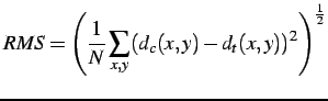 |
(4.2.1) |
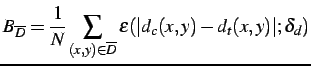
The relative number of the poorly matching
pixels in non-occluded
regions,  , is
defined:
, is
defined:
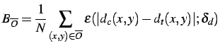 |
(4.2.2) |
where
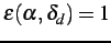 ,
if
,
if  and 0 otherwise.
The relative number of the poorly matching
pixels in textureless
regions,  , is
defined:
, is
defined:
 |
(4.2.3) |
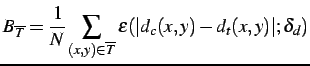
The relative number of the poorly matching
pixels in regions of
discontinuity,  , is
defined:
, is
defined:
 |
(4.2.4) |
Definitions of the texturless,
, occluded,
and depth discontinuity,
,
regions
take account of results of pre-processing of
reference images and ground truth disparity [4]. The textureless
region is that where the squared horizontal intensity gradient
averaged over a square window of a given size is below a given
threshold; the occluded region appears where the forward mapped
disparity lands at a location of a larger disparity; the depth
discontinuity region includes pixels whose neighboring disparity
differ by more than a threshold [4].
An alternative method for evaluating the
accuracy of a stereo
reconstruction was used when there no ground truth is available. In
this case, a qualitative evaluation uses the estimated disparity map to
warp a reference image to a new view, and
compares the resulting image to the actual image from the new
viewpoint [4].
NCSM-SDPS and NCSM-ITER algorithms were
tested on six stereo pairs.
Below, examples of the first step of the NCSM based on two different
noise
estimation methods were illustrated for each stereo pair below by
using  -slices of
the candidate volumes. The empirical noise distributions for these
images were computed using the known ground truth.
The subsequent surface fitting step was shown also by the -slices
compared to ideal
surfaces representing the known ground truth. The final disparity
maps obtained by NCSM algorithms were compared to maps reconstructed
by other stereo algorithms.
-slices of
the candidate volumes. The empirical noise distributions for these
images were computed using the known ground truth.
The subsequent surface fitting step was shown also by the -slices
compared to ideal
surfaces representing the known ground truth. The final disparity
maps obtained by NCSM algorithms were compared to maps reconstructed
by other stereo algorithms.
The stereo pair, `Tsukuba', in Figure
originally
prepared by Ohta and Nakamura, is a real indoor scene with
several distinct layers of disparity. Object boundaries are
relatively complex, e.g. the long thin structure of the lamp's arm.
Figure
shows the distribution of noise for
`Tsukuba'.
Many of the algorithms cannot accurately find these
disparities [
4].
Results for this stereo pair have already been shown in
Chapter
along with the description of NCSM
algorithms.
Figure:
Colour stereo pair, `Tsukuba': Image size:
384x228;
Disparity range: [0-14].
![\includegraphics[width=3.3cm]{mb/tsukuba/tsukuba-l.ppm.eps}](img496.png) |
![\includegraphics[width=3.3cm]{mb/tsukuba/tsukuba-r.ppm.eps}](img497.png) |
![\includegraphics[width=3.3cm]{mb/tsukuba/tsukuba-disp.pgm.eps}](img498.png) |
| Left Image |
Right
Image |
Ground
Truth |
|
Figure:
Empirical noise distribution for `Tsukuba';
overall error range: [-207, 205]; mean absolute error
 :
6.4; standard deviation of absolute errors
:
6.4; standard deviation of absolute errors  : 15.
: 15.
|
|
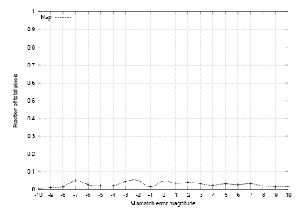
The greyscale stereo pair, `Map', in
Figure
has two highly
textured and slanted surfaces. The matching difficulties result
from a significant occlusion on the background surface because of
relatively large disparity difference between the two surfaces.
Figure shows the distribution of noise for
`Map': note that
most of pixels in this stereo pair do not match because of geometric
and optical distortions caused by large occlusions.
Figure
shows ideal -slices
surfaces of `Map' based
on its ground truth disparity map. Figures and
present candidate volumes and surface fitting
produced by NCSM-SDPS and NCSM-ITER, respectively.
Figure:
Grey stereo pair, `Map': Image size: 284x216;
Disparity range: [0-29].
![\includegraphics[width=2.7cm]{mb/map/map-l.pgm.eps}](img502.png) |
![\includegraphics[width=2.7cm]{mb/map/map-r.pgm.eps}](img503.png) |
![\includegraphics[width=2.7cm]{mb/map/map-disp.pgm.eps}](img504.png) |
| Left Image |
Right
Image |
Ground
Truth |
|
Figure:
Empirical noise distribution for `Map';
overall error range: [-116, 176]; mean absolute error
:
14.7; standard deviation of absolute errors : 20.
|
|
Figure:
Ideal surfaces from the ground truth disparity map.
Stereo pair: 'Map'.
|
|
Figure:
-slices
of candidate corresponding volumes. Stereo pair: `Map';
Algorithms: NCSM-SDPS and NCSM-ITER.
|
|
Figure:
-slices
found from surface fitting. Stereo pair: `Map';
Algorithms: NCSM-SDPS and NCSM-ITER.
|
|
The stereo pair, `Sawtooth', in
Figure
includes three
textured slanted planes with a blue textureless background. Matching
problems occur along the edges of slanted planes.
Figure shows the distribution of noise for
`Sawtooth'.
Figure
illustrates ideal surfaces of the `Sawtooth'
based on its ground truth disparity map. Figures and
present candidate volumes and surface fitting
produced by NCSM-SDPS and NCSM-ITER, respectively.
Figure:
Colour stereo pair, `Sawtooth': Image size:
434x380;
Disparity range: [0-29].
![\includegraphics[width=3.5cm]{mb/sawtooth/sawtooth-l.ppm.eps}](img554.png) |
![\includegraphics[width=3.5cm]{mb/sawtooth/sawtooth-r.ppm.eps}](img555.png) |
![\includegraphics[width=3.5cm]{mb/sawtooth/sawtooth-disp.pgm.eps}](img556.png) |
| Left Image |
Right
Image |
Ground
Truth |
|
Figure:
Empirical noise distribution for `Sawtooth';
overall error range: [-189, 148]; mean absolute error
:
6.2; standard deviation of absolute errors : 15.
|
|
Figure:
Ideal surfaces from the ground truth disparity map.
Stereo pair: `Sawtooth'
|
|
Figure:
-slices
of candidate corresponding volumes. Stereo pair: `Sawtooth';
Algorithms: NCSM-SDPS and NCSM-ITER.
|
|
Figure:
-slices
found from surface fitting. Stereo pair: `Sawtooth';
Algorithms: NCSM-SDPS and NCSM-ITER.
|
|
The stereo pair, `Venus', in Figure is very similar
to
`Sawtooth' and meets with the same matching problems. `Venus' includes
more regions with virtually no texture, and a clear edge shared by
two of the surfaces.
Figure shows the distribution of noise for
`Venus'.
Figure
illustrates ideal
surfaces of `Venus' based on its ground truth disparity map.
Figures
and
present candidate volumes
and surface fitting produced by NCSM-SDPS and NCSM-ITER,
respectively.
Figure:
Colour stereo pair, `Venus': Image size:
434x380;
Disparity range: [0-29].
![\includegraphics[width=3.5cm]{mb/venus/venus-l.ppm.eps}](img636.png) |
![\includegraphics[width=3.5cm]{mb/venus/venus-r.ppm.eps}](img637.png) |
![\includegraphics[width=3.5cm]{mb/venus/venus-disp.pgm.eps}](img638.png) |
| Left Image |
Right
Image |
Ground
Truth |
|
Figure:
Empirical noise distribution for `Venus';
overall error range: [-167, 128]; mean absolute error
:
4.9; standard deviation of absolute errors : 12.
|
|
Figure:
Ideal surfaces from the ground truth disparity map.
Stereo pair: `Venus'.
|
|
Figure:
-slices
of candidate corresponding volumes. Stereo pair: `Venus';
Algorithms: NCSM-SDPS and NCSM-ITER.
|
|
Figure:
-slices
found from surface fitting. Stereo pair: `Venus';
Algorithms: NCSM-SDPS and NCSM-ITER.
|
|
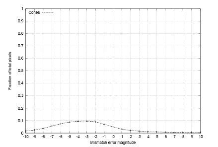
The stereo pair, `Cones', in Figure is one of two
new
stereo sets in the Middlebury database [76] with more
complicated surfaces. Since the previous four stereo sets are too
simple to easily discriminate between more and more advanced
algorithms, the stereo pair, `Cones', with a large disparity range
includes much more textureless areas, curved surfaces and thin
foreground objects in order to challenge stereo algorithms.
Figure shows the distribution of noise for
`Cones', and
for space limitations, Figure
illustrates only the main ideal surfaces for the `Cones' based on its
ground truth disparity map. Also, Figures and
present candidate volumes and surface fitting
produced by NCSM-SDPS and NCSM-ITER, respectively.
Figure:
Colour stereo pair, `Cones': Image size:
450x375;
Disparity range:[0-59].
![\includegraphics[width=4cm]{mb/cones/cones-l.ppm.eps}](img715.png) |
![\includegraphics[width=4cm]{mb/cones/cones-r.ppm.eps}](img716.png) |
![\includegraphics[width=4cm]{mb/cones/cones-disp.pgm.eps}](img717.png) |
| Left Image |
Right
Image |
Ground
Truth |
|
Figure:
Empirical noise distribution for `Cones';
overall error range: [-188, 181]; mean absolute error
:
9.8; standard deviation of absolute errors : 17.
|
|
Figure:
Ideal surfaces from the ground truth
disparity map.
Stereo pair: `Cones'.
|
|
Figure:
-slices
of candidate corresponding volumes. Stereo pair: `Cones';
Algorithms: NCSM-SDPS and NCSM-ITER.
|
|
Figure:
-slices
found from surface fitting. Stereo pair: `Cones';
Algorithms: NCSM-SDPS and NCSM-ITER.
|
|
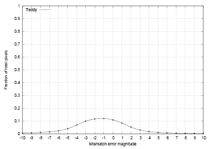
The stereo pair, `Teddy', in Figure
is the second new
complicated scene with a large disparity range including a large
number of surfaces and more complex structures from soft toys and
plants.
Figure
shows the distribution of noise for
`Teddy'.
Figure
illustrates only the main ideal surfaces
of `Teddy' based on its ground truth disparity map. Also,
Figures
and
present candidate volumes
and surface fitting produced by NCSM-SDPS and NCSM-ITER,
respectively.
Figure:
Colour stereo pair, `Teddy': Image size:
450x375;
Disparity range: [0-59].
![\includegraphics[width=4cm]{mb/teddy/teddy-l.ppm.eps}](img834.png) |
![\includegraphics[width=4cm]{mb/teddy/teddy-r.ppm.eps}](img835.png) |
![\includegraphics[width=4cm]{mb/teddy/teddy-disp.pgm.eps}](img836.png) |
| Left Image |
Right
Image |
Ground
Truth |
|
Figure:
Empirical noise distribution for `Teddy';
overall error range: [-209, 195]; mean absolute error
:
7.5; standard deviation of absolute errors : 19.
|
|
Figure:
Ideal surfaces from the ground truth
disparity map.
Stereo pair: `Teddy'.
|
|
Figure:
-slices
of candidate corresponding volumes. Stereo pair: `Teddy';
Algorithms: NCSM-SDPS and NCSM-ITER.
|
|
Figure:
-slices
found from surface fitting. Stereo pair: `Teddy';
Algorithms: NCSM-SDPS and NCSM-ITER.
|
|
Figure
show the true disparity maps for
these six stereo pairs along with the disparity maps reconstructed
using NCSM-SDPS, NCSM-ITER, Graph Minimum Cut with occlusions
(GCO) [1],
Symmetric Belief Propagation
(SBP) [54],
Maximum Flow/Minimum Cut (MCS) [45] and
Symmetric Dynamic Programming Stereo (SDPS) [40]
algorithms.
The performance of these algorithms
according to the evaluation
metrics of Section 4.2 but with some differences is shown in
Table . The ``nonocc'' entry presents the
percentage of ``bad" pixels only in non-occluded regions. Compared
to the ''nonocc'' entry, the ``all'' entry includes partially
occluded regions, and the ``dist'' entry presents the percentage of
``bad" pixels for the regions near depth discontinuities, occluded
and border regions. Also, the pairs, `Cones' and `Teddy', replaced
the previously used pairs, `Map' and `Sawtooth', in order to
evaluate the performance on complex 3D structures with a large
disparity range. Detailed analysis of the experimental results show
that the NCSM framework yields strongly competitive results compared
to the best-performing conventional algorithms on test stereo pairs,
except `Venus' and `Cones', which have many slanted and curved
surfaces. The reason is that the surface fitting approach in
NCSM-SDPS and NCSM-ITER, to date, has been restricted, for
simplicity, to only surface patches, and thus it handles slanted
surfaces relatively poorly. More general surface fitting technique
should overcome this drawback.
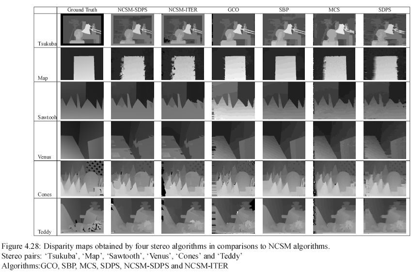
Table 4.1:
Noise-driven concurrent stereo matching (NCSM) algorithms
compare to other stereo algorithms.
Stereo pairs:
`Tsukuba', `Venus', `Cones' and `Teddy'
Algorithms:GCO, SBP, MCS, SDPS, NCSM-SDPS and NCSM-ITER
| % errors of the `bad' matching |
| Algorithm
|
Tsukuba |
Venus |
|
|
nonocc  |
all  |
disc  |
nonocc |
all |
disc |
| GCO
|
1.2 |
2.0 |
6.2 |
1.6 |
2.2 |
6.8 |
| SBP
|
1.0 |
1.8 |
5.1 |
0.2 |
0.3 |
2.2 |
| MCS
|
3.5 |
4.5 |
16.1 |
2.3 |
3.8 |
17.2 |
| SDPS
|
4.2 |
6.0 |
18.1 |
5.2 |
6.5 |
27.5 |
| NCSM-SDPS
|
4.6
|
5.1
|
14.4
|
13.1
|
13.4
|
21.2
|
| NCSM-ITER
|
2.2
|
2.6
|
10.7
|
10.2
|
10.6
|
21.3
|
| Algorithm
|
Cones |
Teddy |
|
|
nonocc |
all |
disc |
nonocc |
all |
disc |
| GCO
|
5.4 |
12.4 |
13.0 |
11.2 |
17.4 |
19.8 |
| SBP
|
4.8 |
10.7 |
10.9 |
6.5 |
10.7 |
17.0 |
| MCS
|
9.4 |
14.5 |
20.8 |
9.3 |
13.9 |
17.9 |
| SDPS
|
11.6 |
16.5 |
23.7 |
10.6 |
14.7 |
21.0 |
| NCSM-SDPS
|
14.7
|
18.6
|
24.7
|
16.2
|
13.4
|
19.8
|
| NCSM-ITER
|
10.5
|
15.6
|
17.3
|
11.7
|
14.1
|
18.1
|
| |
| the
percentage of `bad' pixels in non-occluded regions |
| the
percentage of `bad' pixels in occluded regions |
| the
percentage of `bad' pixels near depth discontinuities, |
| occluded and border regions |
|
|
|
|
|
|
|
Figure
presents 3D reconstruction views of these
test sets. The first column lists all 3D reconstruction results
based on ground truth disparity maps, and the second column and the
third column include the results from NCSM-SDPS and NCSM-ITER
disparity maps, respectively.
Figure:
3D reconstruction according to disparity maps.
Stereo pairs: `Tsukuba', `Map', `Sawtooth',
`Venus', `Cones' and `Teddy'
Disparity maps:
Ground Truth, NCSM-SDPS and NCSM-ITER
|
Ground Truth |
NCSM-SDPS |
NCSM-ITER |
| Tsukuba |
![\includegraphics[width=3.3cm]{mb/3d/tsukuba-true.bmp.eps}](img1017.png) |
![\includegraphics[width=3.3cm]{mb/3d/tsukuba-ncsm-sdps.bmp.eps}](img1018.png) |
![\includegraphics[width=3.3cm]{mb/3d/tsukuba-ncsm-iter.bmp.eps}](img1019.png) |
| Map |
![\includegraphics[width=3.3cm]{mb/3d/map-true.bmp.eps}](img1020.png) |
![\includegraphics[width=3.3cm]{mb/3d/map-ncsm-sdps.bmp.eps}](img1021.png) |
![\includegraphics[width=3.3cm]{mb/3d/map-ncsm-iter.bmp.eps}](img1022.png) |
| Sawtooh |
![\includegraphics[width=3.3cm]{mb/3d/sawtooth-true.bmp.eps}](img1023.png) |
![\includegraphics[width=3.3cm]{mb/3d/sawtooth-ncsm-sdps.bmp.eps}](img1024.png) |
|
| Venus |
![\includegraphics[width=3.3cm]{mb/3d/venus-true.bmp.eps}](img1025.png) |
![\includegraphics[width=3.3cm]{mb/3d/venus-ncsm-sdps.bmp.eps}](img1026.png) |
![\includegraphics[width=3.3cm]{mb/3d/venus-ncsm-iter.bmp.eps}](img1027.png) |
| Teddy |
![\includegraphics[width=3.3cm]{mb/3d/teddy-true.bmp.eps}](img1028.png) |
![\includegraphics[width=3.3cm]{mb/3d/teddy-ncsm-sdps.bmp.eps}](img1029.png) |
![\includegraphics[width=3.3cm]{mb/3d/teddy-ncsm-iter.bmp.eps}](img1030.png) |
| Cones |
![\includegraphics[width=3.3cm]{mb/3d/cones-true.bmp.eps}](img1031.png) |
![\includegraphics[width=3.3cm]{mb/3d/cones-ncsm-sdps.bmp.eps}](img1032.png) |
![\includegraphics[width=3.3cm]{mb/3d/cones-ncsm-iter.bmp.eps}](img1033.png) |
|
In many practical cases, noisy images can be
described by an additive
noise model, where the
noisy image  is the sum of the true (noiseless) image
 under
contrast,
under
contrast,  ,
and offset,
,
and offset,  ,
deviation and
the noise
,
deviation and
the noise  :
:
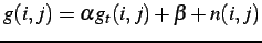 |
(4.4.1) |
In stereo pairs, the noise components in
different pixels are
statistically independent where as
the contrast and offset are limited to a certain range
for adjacent binocularly visible points along with each epipolar line
in NCSM-SDPS or are fixed for all binocularly visible points at the
same disparity level in NCSM-ITER.
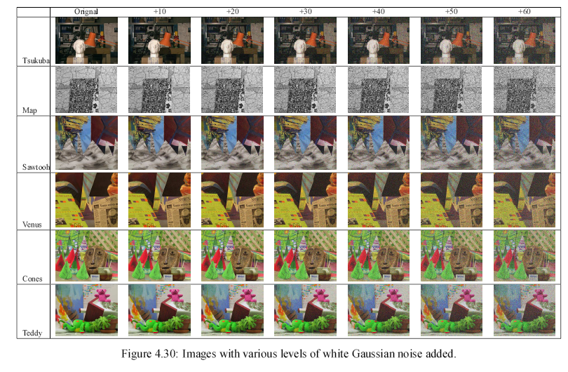
In these experiments,
is an additive Gaussian noise
affecting the right image of a stereo pair. The noise `level' is
defined by the standard deviation. The noisy right images in
Figure
were obtained by increasing
from

to

; the images
becoming more and more grainy with
growing standard deviation.
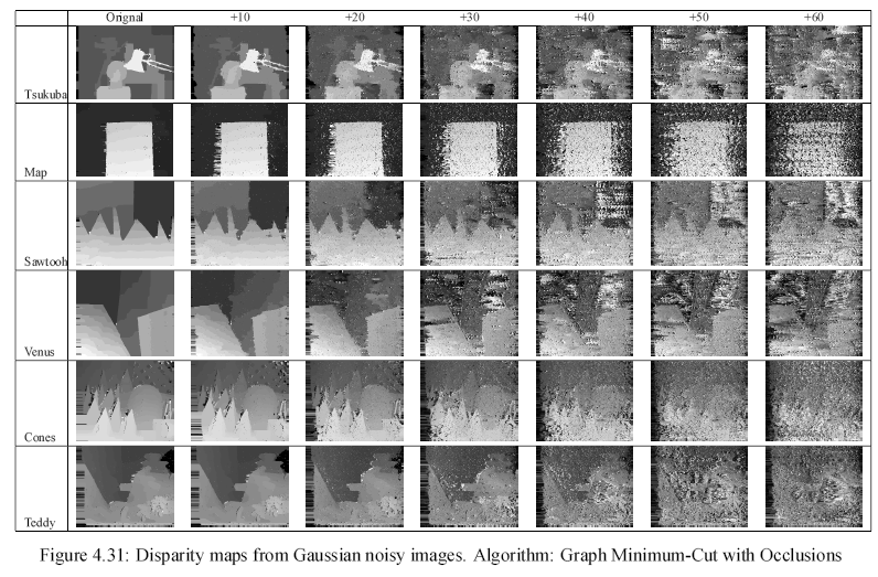
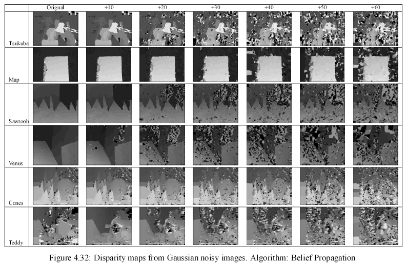
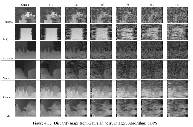
Figure and present
disparity maps obtained by Graph-Cut and Belief Propagation
respectively with stereo pairs distorted by Gaussian noise. The
disparity maps show that these algorithms-the best performers for
images with low noise-completely fail on noisy stereo pairs.
Results from SDPS in Figure are slightly
better, but also fail for high noise. The disparity maps of
NCSM-SDPS and NCSM-ITER in Figures
and
, respectively are visually better and
quite similar, except for `Map' and 'Venus'.
Figure ,
and show the RMS error
plots for each stereo pair under the different noise levels.
Clearly, the RMS's of disparity maps for GC, BP and SDPS increase
rapidly so that these algorithms fail for high noise, but RMS's for
NCSM-SDPS and NCSM-ITER have a slow increase, so that results are
almost same both before and after adding the synthetic noise, even
at quite high noise levels.
Figure:
RMS errors in disparity maps for Gaussian noisy images.
Stereo pairs: `Tsukuba' and 'Map'
|
|
Figure:
RMS errors in disparity maps for Gaussian noisy images.
Stereo pairs: `Sawtooth' and 'Venus'
|
|
Figure:
RMS errors in disparity maps for Gaussian noisy images.
Stereo pairs: `Cones' and 'Teddy'
|
|
Since stereo requires two images-taken by
different cameras or by
the same camera at different times-variations in contrast are a
continuing problem in real systems. In this set of experiment, the
contrast range of the right image of each stereo pair was changed to
a new intensity range, e.g. the transformed right images in
Figure
are obtained by varying the initial image
contrast in the range  .
For example, for a
.
For example, for a  contrast change, the range is shrunk by
  of the total range at each
end,
so that the range
of the total range at each
end,
so that the range ![$ [1,253]$](img1054.png) becomes
becomes
![$ [1+(253-1)\times 0.2, 253- (253-1)\times 0.2] = [51,203]$](img1055.png) .
.
Figure and present
disparity maps obtained by the Graph Minimum-Cut and Belief
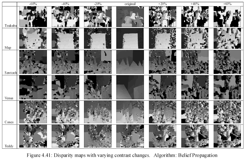
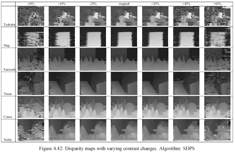
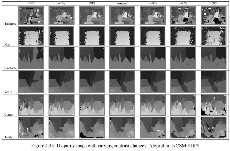
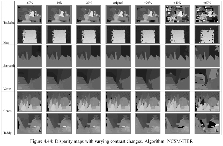
Propagation algorithms with varying contrast differences,
respectively. These algorithms fail for both increased and reduced
contrast range. Figure shows that the
performance of SDPS is slightly better, but also fails with large
contrast
variation. The disparity maps for NCSM-SDPS and NCSM-ITER are shown
in Figures and
respectively. NCSM-ITER works slightly
better than NCSM-SDPS on noisy image pairs of higher contrast.
Figures ,
and plot the RMS error for each stereo
pair. Graph Minimum-cut and Belief Propagation algorithms obviously
fail on noisy image pairs of both higher and lower contrast,
NCSM-SDPS and NCSM-ITER are able to handle these noisy image pairs,
the performance of NCSM-ITER is slightly better than of NCSM-SDPS.
Figure:
RMS error vs degree of contrast change.
Stereo pairs: `Tsukuba' and 'Map'
|
|
Figure:
RMS error vs degree of contrast change.
Stereo pairs: `Sawtooth' and 'Venus'
|
|
Figure:
RMS error vs degree of contrast change.
Stereo pairs: `Cones' and 'Teddy'
|
|
Tables
and
summarise the performance of these algorithms using the metrics of
Section 4.2 for image pairs with an additive fixed Gaussian
noise ( )
and a fixed contrast change ( with
respect to the initial image). Even for
)
and a fixed contrast change ( with
respect to the initial image). Even for
 , which
means that a ``bad" pixel is defined by a very stringent condition:
the RMS between each computed disparity
at position
and the corresponding ground truth disparity
,
is greater than
, which
means that a ``bad" pixel is defined by a very stringent condition:
the RMS between each computed disparity
at position
and the corresponding ground truth disparity
,
is greater than  ,
the NCSM algorithm yields stable results for
stereo pairs with both added noise and contrast changes.
,
the NCSM algorithm yields stable results for
stereo pairs with both added noise and contrast changes.
These results show that, a family of the
NCSM algorithms (NCSM-SDPS
and NCSM-ITER) produces the high quality 3D reconstruction for
various stereo pairs and under different image distortions. The NCSM
framework is generally performs as well as the best-performing
conventional algorithms on the test stereo pairs with no contrast
and offset deviations but notably outperforms these algorithms in
the presence of large contrast deviations and high additive noise.
Table:
Accuracy of NCSM vs other stereo algorithms with
noisy stereo pairs (additive white Gaussian noise,
).
Stereo pairs: `Tsukuba', `Venus', `Cones' and
`Teddy'
Algorithms: GCO, BP, SDPS, NCSM-SDPS and
NCSM-ITER
| % errors of the `bad' matching |
| Algorithm
|
Tsukuba |
Venus |
|
|
nonocc |
all |
disc |
nonocc |
all |
disc |
| GCO
|
41.5 |
42.4 |
47.8 |
56.9 |
57.8 |
62.7 |
| BP
|
35.3 |
36.4 |
39.3 |
51.5 |
51.6 |
47.6 |
| SDPS
|
44.4 |
44.8 |
54.1 |
67.9 |
68.3 |
61.6 |
| NCSM-SDPS
|
21.1 |
21.6 |
37.1 |
48.0 |
48.7 |
53.9 |
| NCSM-ITER
|
12.2 |
12.6 |
23.1 |
40.1 |
40.4 |
33.5 |
| Algorithm
|
Cones |
Teddy |
|
|
nonocc |
all |
disc |
nonocc |
all |
disc |
| GCO
|
35.8 |
37.3 |
45.1 |
56.3 |
58.9 |
52.1 |
| BP
|
33.4 |
36.9 |
41.4 |
50.1 |
52.2 |
48.9 |
| SDPS
|
50.9 |
53.4 |
55.5 |
59.6 |
69.2 |
55.7 |
| NCSM-SDPS
|
26.0 |
29.8 |
35.1 |
19.7 |
22.0 |
28.2 |
| NCSM-ITER
|
16.8 |
20.4 |
34.2 |
24.8 |
27.2 |
21.8 |
|
| the
percentage of `bad' pixels in non-occluded regions |
| the
percentage of `bad' pixels in occluded regions |
| the
percentage of `bad' pixels near depth discontinuities, |
| occluded and border regions |
|
|
|
|
|
|
|
Table:
Accuracy of NCSM vs other stereo algorithms with
noisy stereo pairs (lower contrast change, )
Stereo pairs: `Tsukuba', `Venus', `Cones' and
`Teddy'
Algorithms: GCO, BP, SDPS, NCSM-SDPS and
NCSM-ITER
| % errors of the `bad' matching |
| Algorithm
|
Tsukuba |
Venus |
|
|
nonocc |
all |
disc |
nonocc |
all |
disc |
| GCO
|
59.9 |
61.2 |
68.7 |
49.1 |
48.9 |
62.1 |
| BP
|
68.8 |
69.9 |
71.3 |
56.3 |
56.6 |
70.0 |
| SDPS
|
12.3 |
14.0 |
32.7 |
10.6 |
11.9 |
34.3 |
| NCSM-SDPS
|
13.0 |
13.8 |
35.8 |
20.8 |
21.5 |
33.6 |
| NCSM-ITER
|
5.6 |
6.1 |
16.3 |
21.7 |
21.3 |
35.7 |
| Algorithm
|
Cones |
Teddy |
|
|
nonocc |
all |
disc |
nonocc |
all |
disc |
| GCO
|
56.2 |
58.9 |
63.7 |
66.9 |
68.6 |
72.1 |
| BP
|
55.1 |
57.2 |
60.3 |
68.8 |
69.9 |
71.3 |
| SDPS
|
13.3 |
18.1 |
26.8 |
13.6 |
17.5 |
23.2 |
| NCSM-SDPS
|
20.5 |
24.5 |
31.8 |
17.3 |
15.0 |
23.5 |
| NCSM-ITER
|
17.1 |
20.9 |
27.0 |
13.4 |
14.2 |
19.8 |
|
|
|
|
|
|
|
![\includegraphics[width=3cm]{mb/map/map_ideasurfaces_at_disp4.pgm.eps}](img514.png)
![\includegraphics[width=3cm]{mb/map/map_ideasurfaces_at_disp22.pgm.eps}](img515.png)
![\includegraphics[width=3cm]{mb/map/map_ideasurfaces_at_disp23.pgm.eps}](img516.png)
![\includegraphics[width=3cm]{mb/map/map_ideasurfaces_at_disp24.pgm.eps}](img517.png)
![\includegraphics[width=3cm]{mb/map/map_ideasurfaces_at_disp25.pgm.eps}](img518.png)
![\includegraphics[width=3cm]{mb/map/map_ideasurfaces_at_disp26.pgm.eps}](img519.png)
![\includegraphics[width=3cm]{mb/map/map_ideasurfaces_at_disp27.pgm.eps}](img520.png)
![\includegraphics[width=3cm]{mb/map/map_ideasurfaces_at_disp28.pgm.eps}](img521.png)
![\includegraphics[width=3cm]{mb/map/sdps/20-confidenceMap_at_4.pgm.eps}](img522.png)
![\includegraphics[width=3cm]{mb/map/sdps/20-confidenceMap_at_22.pgm.eps}](img523.png)
![\includegraphics[width=3cm]{mb/map/sdps/20-confidenceMap_at_23.pgm.eps}](img524.png)
![\includegraphics[width=3cm]{mb/map/sdps/20-confidenceMap_at_24.pgm.eps}](img525.png)
![\includegraphics[width=3cm]{mb/map/sdps/20-confidenceMap_at_25.pgm.eps}](img526.png)
![\includegraphics[width=3cm]{mb/map/sdps/20-confidenceMap_at_26.pgm.eps}](img527.png)
![\includegraphics[width=3cm]{mb/map/sdps/20-confidenceMap_at_27.pgm.eps}](img528.png)
![\includegraphics[width=3cm]{mb/map/sdps/20-confidenceMap_at_28.pgm.eps}](img529.png)
![\includegraphics[width=3cm]{mb/map/iter/21-confidenceMap_at_4.pgm.eps}](img530.png)
![\includegraphics[width=3cm]{mb/map/iter/21-confidenceMap_at_22.pgm.eps}](img531.png)
![\includegraphics[width=3cm]{mb/map/iter/21-confidenceMap_at_23.pgm.eps}](img532.png)
![\includegraphics[width=3cm]{mb/map/iter/21-confidenceMap_at_24.pgm.eps}](img533.png)
![\includegraphics[width=3cm]{mb/map/iter/21-confidenceMap_at_25.pgm.eps}](img534.png)
![\includegraphics[width=3cm]{mb/map/iter/21-confidenceMap_at_26.pgm.eps}](img535.png)
![\includegraphics[width=3cm]{mb/map/iter/21-confidenceMap_at_27.pgm.eps}](img536.png)
![\includegraphics[width=3cm]{mb/map/iter/21-confidenceMap_at_28.pgm.eps}](img537.png)
![\includegraphics[width=3cm]{mb/map/sdps/20-surfacefitting_at_4.pgm.eps}](img538.png)
![\includegraphics[width=3cm]{mb/map/sdps/20-surfacefitting_at_22.pgm.eps}](img539.png)
![\includegraphics[width=3cm]{mb/map/sdps/20-surfacefitting_at_23.pgm.eps}](img540.png)
![\includegraphics[width=3cm]{mb/map/sdps/20-surfacefitting_at_24.pgm.eps}](img541.png)
![\includegraphics[width=3cm]{mb/map/sdps/20-surfacefitting_at_25.pgm.eps}](img542.png)
![\includegraphics[width=3cm]{mb/map/sdps/20-surfacefitting_at_26.pgm.eps}](img543.png)
![\includegraphics[width=3cm]{mb/map/sdps/20-surfacefitting_at_27.pgm.eps}](img544.png)
![\includegraphics[width=3cm]{mb/map/sdps/20-surfacefitting_at_28.pgm.eps}](img545.png)
![\includegraphics[width=3cm]{mb/map/iter/21-surfacefitting_at_4.pgm.eps}](img546.png)
![\includegraphics[width=3cm]{mb/map/iter/21-surfacefitting_at_22.pgm.eps}](img547.png)
![\includegraphics[width=3cm]{mb/map/iter/21-surfacefitting_at_23.pgm.eps}](img548.png)
![\includegraphics[width=3cm]{mb/map/iter/21-surfacefitting_at_24.pgm.eps}](img549.png)
![\includegraphics[width=3cm]{mb/map/iter/21-surfacefitting_at_25.pgm.eps}](img550.png)
![\includegraphics[width=3cm]{mb/map/iter/21-surfacefitting_at_26.pgm.eps}](img551.png)
![\includegraphics[width=3cm]{mb/map/iter/21-surfacefitting_at_27.pgm.eps}](img552.png)
![\includegraphics[width=3cm]{mb/map/iter/21-surfacefitting_at_28.pgm.eps}](img553.png)
![\includegraphics[width=2.5cm]{mb/sawtooth/sawtooth_ideasurfaces_at_disp3.pgm.eps}](img561.png)
![\includegraphics[width=2.5cm]{mb/sawtooth/sawtooth_ideasurfaces_at_disp4.pgm.eps}](img562.png)
![\includegraphics[width=2.5cm]{mb/sawtooth/sawtooth_ideasurfaces_at_disp5.pgm.eps}](img563.png)
![\includegraphics[width=2.5cm]{mb/sawtooth/sawtooth_ideasurfaces_at_disp6.pgm.eps}](img564.png)
![\includegraphics[width=2.5cm]{mb/sawtooth/sawtooth_ideasurfaces_at_disp7.pgm.eps}](img565.png)
![\includegraphics[width=2.5cm]{mb/sawtooth/sawtooth_ideasurfaces_at_disp8.pgm.eps}](img566.png)
![\includegraphics[width=2.5cm]{mb/sawtooth/sawtooth_ideasurfaces_at_disp9.pgm.eps}](img567.png)
![\includegraphics[width=2.5cm]{mb/sawtooth/sawtooth_ideasurfaces_at_disp10.pgm.eps}](img568.png)
![\includegraphics[width=2.5cm]{mb/sawtooth/sawtooth_ideasurfaces_at_disp11.pgm.eps}](img569.png)
![\includegraphics[width=2.5cm]{mb/sawtooth/sawtooth_ideasurfaces_at_disp12.pgm.eps}](img570.png)
![\includegraphics[width=2.5cm]{mb/sawtooth/sawtooth_ideasurfaces_at_disp13.pgm.eps}](img571.png)
![\includegraphics[width=2.5cm]{mb/sawtooth/sawtooth_ideasurfaces_at_disp14.pgm.eps}](img572.png)
![\includegraphics[width=2.5cm]{mb/sawtooth/sawtooth_ideasurfaces_at_disp15.pgm.eps}](img573.png)
![\includegraphics[width=2.5cm]{mb/sawtooth/sawtooth_ideasurfaces_at_disp16.pgm.eps}](img574.png)
![\includegraphics[width=2.5cm]{mb/sawtooth/sawtooth_ideasurfaces_at_disp17.pgm.eps}](img575.png)
![\includegraphics[width=2.5cm]{mb/sawtooth/sdps/30-confidenceMap_at_3.pgm.eps}](img576.png)
![\includegraphics[width=2.5cm]{mb/sawtooth/sdps/30-confidenceMap_at_4.pgm.eps}](img577.png)
![\includegraphics[width=2.5cm]{mb/sawtooth/sdps/30-confidenceMap_at_5.pgm.eps}](img578.png)
![\includegraphics[width=2.5cm]{mb/sawtooth/sdps/30-confidenceMap_at_6.pgm.eps}](img579.png)
![\includegraphics[width=2.5cm]{mb/sawtooth/sdps/30-confidenceMap_at_7.pgm.eps}](img580.png)
![\includegraphics[width=2.5cm]{mb/sawtooth/sdps/30-confidenceMap_at_8.pgm.eps}](img581.png)
![\includegraphics[width=2.5cm]{mb/sawtooth/sdps/30-confidenceMap_at_9.pgm.eps}](img582.png)
![\includegraphics[width=2.5cm]{mb/sawtooth/sdps/30-confidenceMap_at_10.pgm.eps}](img583.png)
![\includegraphics[width=2.5cm]{mb/sawtooth/sdps/30-confidenceMap_at_11.pgm.eps}](img584.png)
![\includegraphics[width=2.5cm]{mb/sawtooth/sdps/30-confidenceMap_at_12.pgm.eps}](img585.png)
![\includegraphics[width=2.5cm]{mb/sawtooth/sdps/30-confidenceMap_at_13.pgm.eps}](img586.png)
![\includegraphics[width=2.5cm]{mb/sawtooth/sdps/30-confidenceMap_at_14.pgm.eps}](img587.png)
![\includegraphics[width=2.5cm]{mb/sawtooth/sdps/30-confidenceMap_at_15.pgm.eps}](img588.png)
![\includegraphics[width=2.5cm]{mb/sawtooth/sdps/30-confidenceMap_at_16.pgm.eps}](img589.png)
![\includegraphics[width=2.5cm]{mb/sawtooth/sdps/30-confidenceMap_at_17.pgm.eps}](img590.png)
![\includegraphics[width=2.5cm]{mb/sawtooth/iter/31-confidenceMap_at_3.pgm.eps}](img591.png)
![\includegraphics[width=2.5cm]{mb/sawtooth/iter/31-confidenceMap_at_4.pgm.eps}](img592.png)
![\includegraphics[width=2.5cm]{mb/sawtooth/iter/31-confidenceMap_at_5.pgm.eps}](img593.png)
![\includegraphics[width=2.5cm]{mb/sawtooth/iter/31-confidenceMap_at_6.pgm.eps}](img594.png)
![\includegraphics[width=2.5cm]{mb/sawtooth/iter/31-confidenceMap_at_7.pgm.eps}](img595.png)
![\includegraphics[width=2.5cm]{mb/sawtooth/iter/31-confidenceMap_at_8.pgm.eps}](img596.png)
![\includegraphics[width=2.5cm]{mb/sawtooth/iter/31-confidenceMap_at_9.pgm.eps}](img597.png)
![\includegraphics[width=2.5cm]{mb/sawtooth/iter/31-confidenceMap_at_10.pgm.eps}](img598.png)
![\includegraphics[width=2.5cm]{mb/sawtooth/iter/31-confidenceMap_at_11.pgm.eps}](img599.png)
![\includegraphics[width=2.5cm]{mb/sawtooth/iter/31-confidenceMap_at_12.pgm.eps}](img600.png)
![\includegraphics[width=2.5cm]{mb/sawtooth/iter/31-confidenceMap_at_13.pgm.eps}](img601.png)
![\includegraphics[width=2.5cm]{mb/sawtooth/iter/31-confidenceMap_at_14.pgm.eps}](img602.png)
![\includegraphics[width=2.5cm]{mb/sawtooth/iter/31-confidenceMap_at_15.pgm.eps}](img603.png)
![\includegraphics[width=2.5cm]{mb/sawtooth/iter/31-confidenceMap_at_16.pgm.eps}](img604.png)
![\includegraphics[width=2.5cm]{mb/sawtooth/iter/31-confidenceMap_at_17.pgm.eps}](img605.png)
![\includegraphics[width=2.5cm]{mb/sawtooth/sdps/30-surfacefitting_at_3.pgm.eps}](img606.png)
![\includegraphics[width=2.5cm]{mb/sawtooth/sdps/30-surfacefitting_at_4.pgm.eps}](img607.png)
![\includegraphics[width=2.5cm]{mb/sawtooth/sdps/30-surfacefitting_at_5.pgm.eps}](img608.png)
![\includegraphics[width=2.5cm]{mb/sawtooth/sdps/30-surfacefitting_at_6.pgm.eps}](img609.png)
![\includegraphics[width=2.5cm]{mb/sawtooth/sdps/30-surfacefitting_at_7.pgm.eps}](img610.png)
![\includegraphics[width=2.5cm]{mb/sawtooth/sdps/30-surfacefitting_at_8.pgm.eps}](img611.png)
![\includegraphics[width=2.5cm]{mb/sawtooth/sdps/30-surfacefitting_at_9.pgm.eps}](img612.png)
![\includegraphics[width=2.5cm]{mb/sawtooth/sdps/30-surfacefitting_at_10.pgm.eps}](img613.png)
![\includegraphics[width=2.5cm]{mb/sawtooth/sdps/30-surfacefitting_at_11.pgm.eps}](img614.png)
![\includegraphics[width=2.5cm]{mb/sawtooth/sdps/30-surfacefitting_at_12.pgm.eps}](img615.png)
![\includegraphics[width=2.5cm]{mb/sawtooth/sdps/30-surfacefitting_at_13.pgm.eps}](img616.png)
![\includegraphics[width=2.5cm]{mb/sawtooth/sdps/30-surfacefitting_at_14.pgm.eps}](img617.png)
![\includegraphics[width=2.5cm]{mb/sawtooth/sdps/30-surfacefitting_at_15.pgm.eps}](img618.png)
![\includegraphics[width=2.5cm]{mb/sawtooth/sdps/30-surfacefitting_at_16.pgm.eps}](img619.png)
![\includegraphics[width=2.5cm]{mb/sawtooth/sdps/30-surfacefitting_at_17.pgm.eps}](img620.png)
![\includegraphics[width=2.5cm]{mb/sawtooth/iter/31-surfacefitting_at_3.pgm.eps}](img621.png)
![\includegraphics[width=2.5cm]{mb/sawtooth/iter/31-surfacefitting_at_4.pgm.eps}](img622.png)
![\includegraphics[width=2.5cm]{mb/sawtooth/iter/31-surfacefitting_at_5.pgm.eps}](img623.png)
![\includegraphics[width=2.5cm]{mb/sawtooth/iter/31-surfacefitting_at_6.pgm.eps}](img624.png)
![\includegraphics[width=2.5cm]{mb/sawtooth/iter/31-surfacefitting_at_7.pgm.eps}](img625.png)
![\includegraphics[width=2.5cm]{mb/sawtooth/iter/31-surfacefitting_at_8.pgm.eps}](img626.png)
![\includegraphics[width=2.5cm]{mb/sawtooth/iter/31-surfacefitting_at_9.pgm.eps}](img627.png)
![\includegraphics[width=2.5cm]{mb/sawtooth/iter/31-surfacefitting_at_10.pgm.eps}](img628.png)
![\includegraphics[width=2.5cm]{mb/sawtooth/iter/31-surfacefitting_at_11.pgm.eps}](img629.png)
![\includegraphics[width=2.5cm]{mb/sawtooth/iter/31-surfacefitting_at_12.pgm.eps}](img630.png)
![\includegraphics[width=2.5cm]{mb/sawtooth/iter/31-surfacefitting_at_13.pgm.eps}](img631.png)
![\includegraphics[width=2.5cm]{mb/sawtooth/iter/31-surfacefitting_at_14.pgm.eps}](img632.png)
![\includegraphics[width=2.5cm]{mb/sawtooth/iter/31-surfacefitting_at_15.pgm.eps}](img633.png)
![\includegraphics[width=2.5cm]{mb/sawtooth/iter/31-surfacefitting_at_16.pgm.eps}](img634.png)
![\includegraphics[width=2.5cm]{mb/sawtooth/iter/31-surfacefitting_at_17.pgm.eps}](img635.png)

![\includegraphics[width=2.5cm]{mb/venus/venus_ideasurfaces_at_disp3.pgm.eps}](img640.png)
![\includegraphics[width=2.5cm]{mb/venus/venus_ideasurfaces_at_disp4.pgm.eps}](img641.png)
![\includegraphics[width=2.5cm]{mb/venus/venus_ideasurfaces_at_disp5.pgm.eps}](img642.png)
![\includegraphics[width=2.5cm]{mb/venus/venus_ideasurfaces_at_disp6.pgm.eps}](img643.png)
![\includegraphics[width=2.5cm]{mb/venus/venus_ideasurfaces_at_disp7.pgm.eps}](img644.png)
![\includegraphics[width=2.5cm]{mb/venus/venus_ideasurfaces_at_disp8.pgm.eps}](img645.png)
![\includegraphics[width=2.5cm]{mb/venus/venus_ideasurfaces_at_disp9.pgm.eps}](img646.png)
![\includegraphics[width=2.5cm]{mb/venus/venus_ideasurfaces_at_disp10.pgm.eps}](img647.png)
![\includegraphics[width=2.5cm]{mb/venus/venus_ideasurfaces_at_disp11.pgm.eps}](img648.png)
![\includegraphics[width=2.5cm]{mb/venus/venus_ideasurfaces_at_disp12.pgm.eps}](img649.png)
![\includegraphics[width=2.5cm]{mb/venus/venus_ideasurfaces_at_disp13.pgm.eps}](img650.png)
![\includegraphics[width=2.5cm]{mb/venus/venus_ideasurfaces_at_disp14.pgm.eps}](img651.png)
![\includegraphics[width=2.5cm]{mb/venus/venus_ideasurfaces_at_disp15.pgm.eps}](img652.png)
![\includegraphics[width=2.5cm]{mb/venus/venus_ideasurfaces_at_disp16.pgm.eps}](img653.png)
![\includegraphics[width=2.5cm]{mb/venus/venus_ideasurfaces_at_disp17.pgm.eps}](img654.png)
![\includegraphics[width=2.5cm]{mb/venus/sdps/40-confidenceMap_at_3.pgm.eps}](img655.png)
![\includegraphics[width=2.5cm]{mb/venus/sdps/40-confidenceMap_at_4.pgm.eps}](img656.png)
![\includegraphics[width=2.5cm]{mb/venus/sdps/40-confidenceMap_at_5.pgm.eps}](img657.png)
![\includegraphics[width=2.5cm]{mb/venus/sdps/40-confidenceMap_at_6.pgm.eps}](img658.png)
![\includegraphics[width=2.5cm]{mb/venus/sdps/40-confidenceMap_at_7.pgm.eps}](img659.png)
![\includegraphics[width=2.5cm]{mb/venus/sdps/40-confidenceMap_at_8.pgm.eps}](img660.png)
![\includegraphics[width=2.5cm]{mb/venus/sdps/40-confidenceMap_at_9.pgm.eps}](img661.png)
![\includegraphics[width=2.5cm]{mb/venus/sdps/40-confidenceMap_at_10.pgm.eps}](img662.png)
![\includegraphics[width=2.5cm]{mb/venus/sdps/40-confidenceMap_at_11.pgm.eps}](img663.png)
![\includegraphics[width=2.5cm]{mb/venus/sdps/40-confidenceMap_at_12.pgm.eps}](img664.png)
![\includegraphics[width=2.5cm]{mb/venus/sdps/40-confidenceMap_at_13.pgm.eps}](img665.png)
![\includegraphics[width=2.5cm]{mb/venus/sdps/40-confidenceMap_at_14.pgm.eps}](img666.png)
![\includegraphics[width=2.5cm]{mb/venus/sdps/40-confidenceMap_at_15.pgm.eps}](img667.png)
![\includegraphics[width=2.5cm]{mb/venus/sdps/40-confidenceMap_at_16.pgm.eps}](img668.png)
![\includegraphics[width=2.5cm]{mb/venus/sdps/40-confidenceMap_at_17.pgm.eps}](img669.png)
![\includegraphics[width=2.5cm]{mb/venus/iter/41-confidenceMap_at_3.pgm.eps}](img670.png)
![\includegraphics[width=2.5cm]{mb/venus/iter/41-confidenceMap_at_4.pgm.eps}](img671.png)
![\includegraphics[width=2.5cm]{mb/venus/iter/41-confidenceMap_at_5.pgm.eps}](img672.png)
![\includegraphics[width=2.5cm]{mb/venus/iter/41-confidenceMap_at_6.pgm.eps}](img673.png)
![\includegraphics[width=2.5cm]{mb/venus/iter/41-confidenceMap_at_7.pgm.eps}](img674.png)
![\includegraphics[width=2.5cm]{mb/venus/iter/41-confidenceMap_at_8.pgm.eps}](img675.png)
![\includegraphics[width=2.5cm]{mb/venus/iter/41-confidenceMap_at_9.pgm.eps}](img676.png)
![\includegraphics[width=2.5cm]{mb/venus/iter/41-confidenceMap_at_10.pgm.eps}](img677.png)
![\includegraphics[width=2.5cm]{mb/venus/iter/41-confidenceMap_at_11.pgm.eps}](img678.png)
![\includegraphics[width=2.5cm]{mb/venus/iter/41-confidenceMap_at_12.pgm.eps}](img679.png)
![\includegraphics[width=2.5cm]{mb/venus/iter/41-confidenceMap_at_13.pgm.eps}](img680.png)
![\includegraphics[width=2.5cm]{mb/venus/iter/41-confidenceMap_at_14.pgm.eps}](img681.png)
![\includegraphics[width=2.5cm]{mb/venus/iter/41-confidenceMap_at_15.pgm.eps}](img682.png)
![\includegraphics[width=2.5cm]{mb/venus/iter/41-confidenceMap_at_16.pgm.eps}](img683.png)
![\includegraphics[width=2.5cm]{mb/venus/iter/41-confidenceMap_at_17.pgm.eps}](img684.png)
![\includegraphics[width=2.5cm]{mb/venus/sdps/40-surfacefitting_at_3.pgm.eps}](img685.png)
![\includegraphics[width=2.5cm]{mb/venus/sdps/40-surfacefitting_at_4.pgm.eps}](img686.png)
![\includegraphics[width=2.5cm]{mb/venus/sdps/40-surfacefitting_at_5.pgm.eps}](img687.png)
![\includegraphics[width=2.5cm]{mb/venus/sdps/40-surfacefitting_at_6.pgm.eps}](img688.png)
![\includegraphics[width=2.5cm]{mb/venus/sdps/40-surfacefitting_at_7.pgm.eps}](img689.png)
![\includegraphics[width=2.5cm]{mb/venus/sdps/40-surfacefitting_at_8.pgm.eps}](img690.png)
![\includegraphics[width=2.5cm]{mb/venus/sdps/40-surfacefitting_at_9.pgm.eps}](img691.png)
![\includegraphics[width=2.5cm]{mb/venus/sdps/40-surfacefitting_at_10.pgm.eps}](img692.png)
![\includegraphics[width=2.5cm]{mb/venus/sdps/40-surfacefitting_at_11.pgm.eps}](img693.png)
![\includegraphics[width=2.5cm]{mb/venus/sdps/40-surfacefitting_at_12.pgm.eps}](img694.png)
![\includegraphics[width=2.5cm]{mb/venus/sdps/40-surfacefitting_at_13.pgm.eps}](img695.png)
![\includegraphics[width=2.5cm]{mb/venus/sdps/40-surfacefitting_at_14.pgm.eps}](img696.png)
![\includegraphics[width=2.5cm]{mb/venus/sdps/40-surfacefitting_at_15.pgm.eps}](img697.png)
![\includegraphics[width=2.5cm]{mb/venus/sdps/40-surfacefitting_at_16.pgm.eps}](img698.png)
![\includegraphics[width=2.5cm]{mb/venus/sdps/40-surfacefitting_at_17.pgm.eps}](img699.png)
![\includegraphics[width=2.5cm]{mb/venus/iter/41-surfacefitting_at_3.pgm.eps}](img700.png)
![\includegraphics[width=2.5cm]{mb/venus/iter/41-surfacefitting_at_4.pgm.eps}](img701.png)
![\includegraphics[width=2.5cm]{mb/venus/iter/41-surfacefitting_at_5.pgm.eps}](img702.png)
![\includegraphics[width=2.5cm]{mb/venus/iter/41-surfacefitting_at_6.pgm.eps}](img703.png)
![\includegraphics[width=2.5cm]{mb/venus/iter/41-surfacefitting_at_7.pgm.eps}](img704.png)
![\includegraphics[width=2.5cm]{mb/venus/iter/41-surfacefitting_at_8.pgm.eps}](img705.png)
![\includegraphics[width=2.5cm]{mb/venus/iter/41-surfacefitting_at_9.pgm.eps}](img706.png)
![\includegraphics[width=2.5cm]{mb/venus/iter/41-surfacefitting_at_10.pgm.eps}](img707.png)
![\includegraphics[width=2.5cm]{mb/venus/iter/41-surfacefitting_at_11.pgm.eps}](img708.png)
![\includegraphics[width=2.5cm]{mb/venus/iter/41-surfacefitting_at_12.pgm.eps}](img709.png)
![\includegraphics[width=2.5cm]{mb/venus/iter/41-surfacefitting_at_13.pgm.eps}](img710.png)
![\includegraphics[width=2.5cm]{mb/venus/iter/41-surfacefitting_at_14.pgm.eps}](img711.png)
![\includegraphics[width=2.5cm]{mb/venus/iter/41-surfacefitting_at_15.pgm.eps}](img712.png)
![\includegraphics[width=2.5cm]{mb/venus/iter/41-surfacefitting_at_16.pgm.eps}](img713.png)
![\includegraphics[width=2.5cm]{mb/venus/iter/41-surfacefitting_at_17.pgm.eps}](img714.png)
![\includegraphics[width=2.5cm]{mb/cones/cones_ideasurfaces_at_disp0.pgm.eps}](img734.png)
![\includegraphics[width=2.5cm]{mb/cones/cones_ideasurfaces_at_disp17.pgm.eps}](img735.png)
![\includegraphics[width=2.5cm]{mb/cones/cones_ideasurfaces_at_disp20.pgm.eps}](img736.png)
![\includegraphics[width=2.5cm]{mb/cones/cones_ideasurfaces_at_disp21.pgm.eps}](img737.png)
![\includegraphics[width=2.5cm]{mb/cones/cones_ideasurfaces_at_disp23.pgm.eps}](img738.png)
![\includegraphics[width=2.5cm]{mb/cones/cones_ideasurfaces_at_disp24.pgm.eps}](img739.png)
![\includegraphics[width=2.5cm]{mb/cones/cones_ideasurfaces_at_disp25.pgm.eps}](img740.png)
![\includegraphics[width=2.5cm]{mb/cones/cones_ideasurfaces_at_disp28.pgm.eps}](img741.png)
![\includegraphics[width=2.5cm]{mb/cones/cones_ideasurfaces_at_disp30.pgm.eps}](img742.png)
![\includegraphics[width=2.5cm]{mb/cones/cones_ideasurfaces_at_disp32.pgm.eps}](img743.png)
![\includegraphics[width=2.5cm]{mb/cones/cones_ideasurfaces_at_disp34.pgm.eps}](img744.png)
![\includegraphics[width=2.5cm]{mb/cones/cones_ideasurfaces_at_disp36.pgm.eps}](img745.png)
![\includegraphics[width=2.5cm]{mb/cones/cones_ideasurfaces_at_disp38.pgm.eps}](img746.png)
![\includegraphics[width=2.5cm]{mb/cones/cones_ideasurfaces_at_disp40.pgm.eps}](img747.png)
![\includegraphics[width=2.5cm]{mb/cones/cones_ideasurfaces_at_disp43.pgm.eps}](img748.png)
![\includegraphics[width=2.5cm]{mb/cones/cones_ideasurfaces_at_disp44.pgm.eps}](img749.png)
![\includegraphics[width=2.5cm]{mb/cones/cones_ideasurfaces_at_disp46.pgm.eps}](img750.png)
![\includegraphics[width=2.5cm]{mb/cones/cones_ideasurfaces_at_disp48.pgm.eps}](img751.png)
![\includegraphics[width=2.5cm]{mb/cones/cones_ideasurfaces_at_disp51.pgm.eps}](img752.png)
![\includegraphics[width=2.5cm]{mb/cones/cones_ideasurfaces_at_disp53.pgm.eps}](img753.png)
![\includegraphics[width=2.3cm]{mb/cones/sdps/60-confidenceMap_at_0.pgm.eps}](img754.png)
![\includegraphics[width=2.3cm]{mb/cones/sdps/60-confidenceMap_at_17.pgm.eps}](img755.png)
![\includegraphics[width=2.3cm]{mb/cones/sdps/60-confidenceMap_at_20.pgm.eps}](img756.png)
![\includegraphics[width=2.3cm]{mb/cones/sdps/60-confidenceMap_at_21.pgm.eps}](img757.png)
![\includegraphics[width=2.3cm]{mb/cones/sdps/60-confidenceMap_at_23.pgm.eps}](img758.png)
![\includegraphics[width=2.3cm]{mb/cones/sdps/60-confidenceMap_at_24.pgm.eps}](img759.png)
![\includegraphics[width=2.3cm]{mb/cones/sdps/60-confidenceMap_at_25.pgm.eps}](img760.png)
![\includegraphics[width=2.3cm]{mb/cones/sdps/60-confidenceMap_at_28.pgm.eps}](img761.png)
![\includegraphics[width=2.3cm]{mb/cones/sdps/60-confidenceMap_at_30.pgm.eps}](img762.png)
![\includegraphics[width=2.3cm]{mb/cones/sdps/60-confidenceMap_at_32.pgm.eps}](img763.png)
![\includegraphics[width=2.3cm]{mb/cones/sdps/60-confidenceMap_at_34.pgm.eps}](img764.png)
![\includegraphics[width=2.3cm]{mb/cones/sdps/60-confidenceMap_at_36.pgm.eps}](img765.png)
![\includegraphics[width=2.3cm]{mb/cones/sdps/60-confidenceMap_at_38.pgm.eps}](img766.png)
![\includegraphics[width=2.3cm]{mb/cones/sdps/60-confidenceMap_at_40.pgm.eps}](img767.png)
![\includegraphics[width=2.3cm]{mb/cones/sdps/60-confidenceMap_at_43.pgm.eps}](img768.png)
![\includegraphics[width=2.3cm]{mb/cones/sdps/60-confidenceMap_at_44.pgm.eps}](img769.png)
![\includegraphics[width=2.3cm]{mb/cones/sdps/60-confidenceMap_at_46.pgm.eps}](img770.png)
![\includegraphics[width=2.3cm]{mb/cones/sdps/60-confidenceMap_at_48.pgm.eps}](img771.png)
![\includegraphics[width=2.3cm]{mb/cones/sdps/60-confidenceMap_at_51.pgm.eps}](img772.png)
![\includegraphics[width=2.3cm]{mb/cones/sdps/60-confidenceMap_at_53.pgm.eps}](img773.png)
![\includegraphics[width=2.3cm]{mb/cones/iter/61-confidenceMap_at_0.pgm.eps}](img774.png)
![\includegraphics[width=2.3cm]{mb/cones/iter/61-confidenceMap_at_17.pgm.eps}](img775.png)
![\includegraphics[width=2.3cm]{mb/cones/iter/61-confidenceMap_at_20.pgm.eps}](img776.png)
![\includegraphics[width=2.3cm]{mb/cones/iter/61-confidenceMap_at_21.pgm.eps}](img777.png)
![\includegraphics[width=2.3cm]{mb/cones/iter/61-confidenceMap_at_23.pgm.eps}](img778.png)
![\includegraphics[width=2.3cm]{mb/cones/iter/61-confidenceMap_at_24.pgm.eps}](img779.png)
![\includegraphics[width=2.3cm]{mb/cones/iter/61-confidenceMap_at_25.pgm.eps}](img780.png)
![\includegraphics[width=2.3cm]{mb/cones/iter/61-confidenceMap_at_28.pgm.eps}](img781.png)
![\includegraphics[width=2.3cm]{mb/cones/iter/61-confidenceMap_at_30.pgm.eps}](img782.png)
![\includegraphics[width=2.3cm]{mb/cones/iter/61-confidenceMap_at_32.pgm.eps}](img783.png)
![\includegraphics[width=2.3cm]{mb/cones/iter/61-confidenceMap_at_34.pgm.eps}](img784.png)
![\includegraphics[width=2.3cm]{mb/cones/iter/61-confidenceMap_at_36.pgm.eps}](img785.png)
![\includegraphics[width=2.3cm]{mb/cones/iter/61-confidenceMap_at_38.pgm.eps}](img786.png)
![\includegraphics[width=2.3cm]{mb/cones/iter/61-confidenceMap_at_40.pgm.eps}](img787.png)
![\includegraphics[width=2.3cm]{mb/cones/iter/61-confidenceMap_at_43.pgm.eps}](img788.png)
![\includegraphics[width=2.3cm]{mb/cones/iter/61-confidenceMap_at_44.pgm.eps}](img789.png)
![\includegraphics[width=2.3cm]{mb/cones/iter/61-confidenceMap_at_46.pgm.eps}](img790.png)
![\includegraphics[width=2.3cm]{mb/cones/iter/61-confidenceMap_at_48.pgm.eps}](img791.png)
![\includegraphics[width=2.3cm]{mb/cones/iter/61-confidenceMap_at_51.pgm.eps}](img792.png)
![\includegraphics[width=2.3cm]{mb/cones/iter/61-confidenceMap_at_53.pgm.eps}](img793.png)
![\includegraphics[width=2.3cm]{mb/cones/sdps/60-surfacefitting_at_0.pgm.eps}](img794.png)
![\includegraphics[width=2.3cm]{mb/cones/sdps/60-surfacefitting_at_17.pgm.eps}](img795.png)
![\includegraphics[width=2.3cm]{mb/cones/sdps/60-surfacefitting_at_20.pgm.eps}](img796.png)
![\includegraphics[width=2.3cm]{mb/cones/sdps/60-surfacefitting_at_21.pgm.eps}](img797.png)
![\includegraphics[width=2.3cm]{mb/cones/sdps/60-surfacefitting_at_23.pgm.eps}](img798.png)
![\includegraphics[width=2.3cm]{mb/cones/sdps/60-surfacefitting_at_24.pgm.eps}](img799.png)
![\includegraphics[width=2.3cm]{mb/cones/sdps/60-surfacefitting_at_25.pgm.eps}](img800.png)
![\includegraphics[width=2.3cm]{mb/cones/sdps/60-surfacefitting_at_28.pgm.eps}](img801.png)
![\includegraphics[width=2.3cm]{mb/cones/sdps/60-surfacefitting_at_30.pgm.eps}](img802.png)
![\includegraphics[width=2.3cm]{mb/cones/sdps/60-surfacefitting_at_32.pgm.eps}](img803.png)
![\includegraphics[width=2.3cm]{mb/cones/sdps/60-surfacefitting_at_34.pgm.eps}](img804.png)
![\includegraphics[width=2.3cm]{mb/cones/sdps/60-surfacefitting_at_36.pgm.eps}](img805.png)
![\includegraphics[width=2.3cm]{mb/cones/sdps/60-surfacefitting_at_38.pgm.eps}](img806.png)
![\includegraphics[width=2.3cm]{mb/cones/sdps/60-surfacefitting_at_40.pgm.eps}](img807.png)
![\includegraphics[width=2.3cm]{mb/cones/sdps/60-surfacefitting_at_43.pgm.eps}](img808.png)
![\includegraphics[width=2.3cm]{mb/cones/sdps/60-surfacefitting_at_44.pgm.eps}](img809.png)
![\includegraphics[width=2.3cm]{mb/cones/sdps/60-surfacefitting_at_46.pgm.eps}](img810.png)
![\includegraphics[width=2.3cm]{mb/cones/sdps/60-surfacefitting_at_48.pgm.eps}](img811.png)
![\includegraphics[width=2.3cm]{mb/cones/sdps/60-surfacefitting_at_51.pgm.eps}](img812.png)
![\includegraphics[width=2.3cm]{mb/cones/sdps/60-surfacefitting_at_53.pgm.eps}](img813.png)
![\includegraphics[width=2.3cm]{mb/cones/iter/61-surfacefitting_at_0.pgm.eps}](img814.png)
![\includegraphics[width=2.3cm]{mb/cones/iter/61-surfacefitting_at_17.pgm.eps}](img815.png)
![\includegraphics[width=2.3cm]{mb/cones/iter/61-surfacefitting_at_20.pgm.eps}](img816.png)
![\includegraphics[width=2.3cm]{mb/cones/iter/61-surfacefitting_at_21.pgm.eps}](img817.png)
![\includegraphics[width=2.3cm]{mb/cones/iter/61-surfacefitting_at_23.pgm.eps}](img818.png)
![\includegraphics[width=2.3cm]{mb/cones/iter/61-surfacefitting_at_24.pgm.eps}](img819.png)
![\includegraphics[width=2.3cm]{mb/cones/iter/61-surfacefitting_at_25.pgm.eps}](img820.png)
![\includegraphics[width=2.3cm]{mb/cones/iter/61-surfacefitting_at_28.pgm.eps}](img821.png)
![\includegraphics[width=2.3cm]{mb/cones/iter/61-surfacefitting_at_30.pgm.eps}](img822.png)
![\includegraphics[width=2.3cm]{mb/cones/iter/61-surfacefitting_at_32.pgm.eps}](img823.png)
![\includegraphics[width=2.3cm]{mb/cones/iter/61-surfacefitting_at_34.pgm.eps}](img824.png)
![\includegraphics[width=2.3cm]{mb/cones/iter/61-surfacefitting_at_36.pgm.eps}](img825.png)
![\includegraphics[width=2.3cm]{mb/cones/iter/61-surfacefitting_at_38.pgm.eps}](img826.png)
![\includegraphics[width=2.3cm]{mb/cones/iter/61-surfacefitting_at_40.pgm.eps}](img827.png)
![\includegraphics[width=2.3cm]{mb/cones/iter/61-surfacefitting_at_43.pgm.eps}](img828.png)
![\includegraphics[width=2.3cm]{mb/cones/iter/61-surfacefitting_at_44.pgm.eps}](img829.png)
![\includegraphics[width=2.3cm]{mb/cones/iter/61-surfacefitting_at_46.pgm.eps}](img830.png)
![\includegraphics[width=2.3cm]{mb/cones/iter/61-surfacefitting_at_48.pgm.eps}](img831.png)
![\includegraphics[width=2.3cm]{mb/cones/iter/61-surfacefitting_at_51.pgm.eps}](img832.png)
![\includegraphics[width=2.3cm]{mb/cones/iter/61-surfacefitting_at_53.pgm.eps}](img833.png)
![\includegraphics[width=2.5cm]{mb/teddy/teddy_ideasurfaces_at_disp0.pgm.eps}](img844.png)
![\includegraphics[width=2.5cm]{mb/teddy/teddy_ideasurfaces_at_disp15.pgm.eps}](img845.png)
![\includegraphics[width=2.5cm]{mb/teddy/teddy_ideasurfaces_at_disp16.pgm.eps}](img846.png)
![\includegraphics[width=2.5cm]{mb/teddy/teddy_ideasurfaces_at_disp17.pgm.eps}](img847.png)
![\includegraphics[width=2.5cm]{mb/teddy/teddy_ideasurfaces_at_disp18.pgm.eps}](img848.png)
![\includegraphics[width=2.5cm]{mb/teddy/teddy_ideasurfaces_at_disp20.pgm.eps}](img849.png)
![\includegraphics[width=2.5cm]{mb/teddy/teddy_ideasurfaces_at_disp21.pgm.eps}](img850.png)
![\includegraphics[width=2.5cm]{mb/teddy/teddy_ideasurfaces_at_disp22.pgm.eps}](img851.png)
![\includegraphics[width=2.5cm]{mb/teddy/teddy_ideasurfaces_at_disp28.pgm.eps}](img852.png)
![\includegraphics[width=2.5cm]{mb/teddy/teddy_ideasurfaces_at_disp29.pgm.eps}](img853.png)
![\includegraphics[width=2.5cm]{mb/teddy/teddy_ideasurfaces_at_disp30.pgm.eps}](img854.png)
![\includegraphics[width=2.5cm]{mb/teddy/teddy_ideasurfaces_at_disp32.pgm.eps}](img855.png)
![\includegraphics[width=2.5cm]{mb/teddy/teddy_ideasurfaces_at_disp33.pgm.eps}](img856.png)
![\includegraphics[width=2.5cm]{mb/teddy/teddy_ideasurfaces_at_disp34.pgm.eps}](img857.png)
![\includegraphics[width=2.5cm]{mb/teddy/teddy_ideasurfaces_at_disp35.pgm.eps}](img858.png)
![\includegraphics[width=2.5cm]{mb/teddy/teddy_ideasurfaces_at_disp37.pgm.eps}](img859.png)
![\includegraphics[width=2.5cm]{mb/teddy/teddy_ideasurfaces_at_disp38.pgm.eps}](img860.png)
![\includegraphics[width=2.5cm]{mb/teddy/teddy_ideasurfaces_at_disp40.pgm.eps}](img861.png)
![\includegraphics[width=2.5cm]{mb/teddy/teddy_ideasurfaces_at_disp41.pgm.eps}](img862.png)
![\includegraphics[width=2.5cm]{mb/teddy/teddy_ideasurfaces_at_disp43.pgm.eps}](img863.png)
![\includegraphics[width=2.3cm]{mb/teddy/sdps/50-confidenceMap_at_0.pgm.eps}](img865.png)
![\includegraphics[width=2.3cm]{mb/teddy/sdps/50-confidenceMap_at_15.pgm.eps}](img866.png)
![\includegraphics[width=2.3cm]{mb/teddy/sdps/50-confidenceMap_at_16.pgm.eps}](img867.png)
![\includegraphics[width=2.3cm]{mb/teddy/sdps/50-confidenceMap_at_17.pgm.eps}](img868.png)
![\includegraphics[width=2.3cm]{mb/teddy/sdps/50-confidenceMap_at_18.pgm.eps}](img869.png)
![\includegraphics[width=2.3cm]{mb/teddy/sdps/50-confidenceMap_at_20.pgm.eps}](img870.png)
![\includegraphics[width=2.3cm]{mb/teddy/sdps/50-confidenceMap_at_21.pgm.eps}](img871.png)
![\includegraphics[width=2.3cm]{mb/teddy/sdps/50-confidenceMap_at_22.pgm.eps}](img872.png)
![\includegraphics[width=2.3cm]{mb/teddy/sdps/50-confidenceMap_at_28.pgm.eps}](img873.png)
![\includegraphics[width=2.3cm]{mb/teddy/sdps/50-confidenceMap_at_29.pgm.eps}](img874.png)
![\includegraphics[width=2.3cm]{mb/teddy/sdps/50-confidenceMap_at_30.pgm.eps}](img875.png)
![\includegraphics[width=2.3cm]{mb/teddy/sdps/50-confidenceMap_at_32.pgm.eps}](img876.png)
![\includegraphics[width=2.3cm]{mb/teddy/sdps/50-confidenceMap_at_33.pgm.eps}](img877.png)
![\includegraphics[width=2.3cm]{mb/teddy/sdps/50-confidenceMap_at_34.pgm.eps}](img878.png)
![\includegraphics[width=2.3cm]{mb/teddy/sdps/50-confidenceMap_at_35.pgm.eps}](img879.png)
![\includegraphics[width=2.3cm]{mb/teddy/sdps/50-confidenceMap_at_37.pgm.eps}](img880.png)
![\includegraphics[width=2.3cm]{mb/teddy/sdps/50-confidenceMap_at_38.pgm.eps}](img881.png)
![\includegraphics[width=2.3cm]{mb/teddy/sdps/50-confidenceMap_at_40.pgm.eps}](img882.png)
![\includegraphics[width=2.3cm]{mb/teddy/sdps/50-confidenceMap_at_41.pgm.eps}](img883.png)
![\includegraphics[width=2.3cm]{mb/teddy/sdps/50-confidenceMap_at_43.pgm.eps}](img884.png)
![\includegraphics[width=2.3cm]{mb/teddy/iter/51-confidenceMap_at_0.pgm.eps}](img885.png)
![\includegraphics[width=2.3cm]{mb/teddy/iter/51-confidenceMap_at_15.pgm.eps}](img886.png)
![\includegraphics[width=2.3cm]{mb/teddy/iter/51-confidenceMap_at_16.pgm.eps}](img887.png)
![\includegraphics[width=2.3cm]{mb/teddy/iter/51-confidenceMap_at_17.pgm.eps}](img888.png)
![\includegraphics[width=2.3cm]{mb/teddy/iter/51-confidenceMap_at_18.pgm.eps}](img889.png)
![\includegraphics[width=2.3cm]{mb/teddy/iter/51-confidenceMap_at_20.pgm.eps}](img890.png)
![\includegraphics[width=2.3cm]{mb/teddy/iter/51-confidenceMap_at_21.pgm.eps}](img891.png)
![\includegraphics[width=2.3cm]{mb/teddy/iter/51-confidenceMap_at_22.pgm.eps}](img892.png)
![\includegraphics[width=2.3cm]{mb/teddy/iter/51-confidenceMap_at_28.pgm.eps}](img893.png)
![\includegraphics[width=2.3cm]{mb/teddy/iter/51-confidenceMap_at_29.pgm.eps}](img894.png)
![\includegraphics[width=2.3cm]{mb/teddy/iter/51-confidenceMap_at_30.pgm.eps}](img895.png)
![\includegraphics[width=2.3cm]{mb/teddy/iter/51-confidenceMap_at_32.pgm.eps}](img896.png)
![\includegraphics[width=2.3cm]{mb/teddy/iter/51-confidenceMap_at_33.pgm.eps}](img897.png)
![\includegraphics[width=2.3cm]{mb/teddy/iter/51-confidenceMap_at_34.pgm.eps}](img898.png)
![\includegraphics[width=2.3cm]{mb/teddy/iter/51-confidenceMap_at_35.pgm.eps}](img899.png)
![\includegraphics[width=2.3cm]{mb/teddy/iter/51-confidenceMap_at_37.pgm.eps}](img900.png)
![\includegraphics[width=2.3cm]{mb/teddy/iter/51-confidenceMap_at_38.pgm.eps}](img901.png)
![\includegraphics[width=2.3cm]{mb/teddy/iter/51-confidenceMap_at_40.pgm.eps}](img902.png)
![\includegraphics[width=2.3cm]{mb/teddy/iter/51-confidenceMap_at_41.pgm.eps}](img903.png)
![\includegraphics[width=2.3cm]{mb/teddy/iter/51-confidenceMap_at_43.pgm.eps}](img904.png)
![\includegraphics[width=2.3cm]{mb/teddy/sdps/50-surfacefitting_at_0.pgm.eps}](img905.png)
![\includegraphics[width=2.3cm]{mb/teddy/sdps/50-surfacefitting_at_15.pgm.eps}](img906.png)
![\includegraphics[width=2.3cm]{mb/teddy/sdps/50-surfacefitting_at_16.pgm.eps}](img907.png)
![\includegraphics[width=2.3cm]{mb/teddy/sdps/50-surfacefitting_at_17.pgm.eps}](img908.png)
![\includegraphics[width=2.3cm]{mb/teddy/sdps/50-surfacefitting_at_18.pgm.eps}](img909.png)
![\includegraphics[width=2.3cm]{mb/teddy/sdps/50-surfacefitting_at_20.pgm.eps}](img910.png)
![\includegraphics[width=2.3cm]{mb/teddy/sdps/50-surfacefitting_at_21.pgm.eps}](img911.png)
![\includegraphics[width=2.3cm]{mb/teddy/sdps/50-surfacefitting_at_22.pgm.eps}](img912.png)
![\includegraphics[width=2.3cm]{mb/teddy/sdps/50-surfacefitting_at_28.pgm.eps}](img913.png)
![\includegraphics[width=2.3cm]{mb/teddy/sdps/50-surfacefitting_at_29.pgm.eps}](img914.png)
![\includegraphics[width=2.3cm]{mb/teddy/sdps/50-surfacefitting_at_30.pgm.eps}](img915.png)
![\includegraphics[width=2.3cm]{mb/teddy/sdps/50-surfacefitting_at_32.pgm.eps}](img916.png)
![\includegraphics[width=2.3cm]{mb/teddy/sdps/50-surfacefitting_at_33.pgm.eps}](img917.png)
![\includegraphics[width=2.3cm]{mb/teddy/sdps/50-surfacefitting_at_34.pgm.eps}](img918.png)
![\includegraphics[width=2.3cm]{mb/teddy/sdps/50-surfacefitting_at_35.pgm.eps}](img919.png)
![\includegraphics[width=2.3cm]{mb/teddy/sdps/50-surfacefitting_at_37.pgm.eps}](img920.png)
![\includegraphics[width=2.3cm]{mb/teddy/sdps/50-surfacefitting_at_38.pgm.eps}](img921.png)
![\includegraphics[width=2.3cm]{mb/teddy/sdps/50-surfacefitting_at_40.pgm.eps}](img922.png)
![\includegraphics[width=2.3cm]{mb/teddy/sdps/50-surfacefitting_at_41.pgm.eps}](img923.png)
![\includegraphics[width=2.3cm]{mb/teddy/sdps/50-surfacefitting_at_43.pgm.eps}](img924.png)
![\includegraphics[width=2.3cm]{mb/teddy/iter/51-surfacefitting_at_0.pgm.eps}](img925.png)
![\includegraphics[width=2.3cm]{mb/teddy/iter/51-surfacefitting_at_15.pgm.eps}](img926.png)
![\includegraphics[width=2.3cm]{mb/teddy/iter/51-surfacefitting_at_16.pgm.eps}](img927.png)
![\includegraphics[width=2.3cm]{mb/teddy/iter/51-surfacefitting_at_17.pgm.eps}](img928.png)
![\includegraphics[width=2.3cm]{mb/teddy/iter/51-surfacefitting_at_18.pgm.eps}](img929.png)
![\includegraphics[width=2.3cm]{mb/teddy/iter/51-surfacefitting_at_20.pgm.eps}](img930.png)
![\includegraphics[width=2.3cm]{mb/teddy/iter/51-surfacefitting_at_21.pgm.eps}](img931.png)
![\includegraphics[width=2.3cm]{mb/teddy/iter/51-surfacefitting_at_22.pgm.eps}](img932.png)
![\includegraphics[width=2.3cm]{mb/teddy/iter/51-surfacefitting_at_28.pgm.eps}](img933.png)
![\includegraphics[width=2.3cm]{mb/teddy/iter/51-surfacefitting_at_29.pgm.eps}](img934.png)
![\includegraphics[width=2.3cm]{mb/teddy/iter/51-surfacefitting_at_30.pgm.eps}](img935.png)
![\includegraphics[width=2.3cm]{mb/teddy/iter/51-surfacefitting_at_32.pgm.eps}](img936.png)
![\includegraphics[width=2.3cm]{mb/teddy/iter/51-surfacefitting_at_33.pgm.eps}](img937.png)
![\includegraphics[width=2.3cm]{mb/teddy/iter/51-surfacefitting_at_34.pgm.eps}](img938.png)
![\includegraphics[width=2.3cm]{mb/teddy/iter/51-surfacefitting_at_35.pgm.eps}](img939.png)
![\includegraphics[width=2.3cm]{mb/teddy/iter/51-surfacefitting_at_37.pgm.eps}](img940.png)
![\includegraphics[width=2.3cm]{mb/teddy/iter/51-surfacefitting_at_38.pgm.eps}](img941.png)
![\includegraphics[width=2.3cm]{mb/teddy/iter/51-surfacefitting_at_40.pgm.eps}](img942.png)
![\includegraphics[width=2.3cm]{mb/teddy/iter/51-surfacefitting_at_41.pgm.eps}](img943.png)
![\includegraphics[width=2.3cm]{mb/teddy/iter/51-surfacefitting_at_43.pgm.eps}](img944.png)
![\includegraphics[width=13cm]{dpms_noise/excel/tsukuba-g.bmp.eps}](img1045.png)
![\includegraphics[width=13cm]{dpms_noise/excel/map-g.bmp.eps}](img1046.png)
![\includegraphics[width=13cm]{dpms_noise/excel/sawtooth-g.bmp.eps}](img1047.png)
![\includegraphics[width=13cm]{dpms_noise/excel/venus-g.bmp.eps}](img1048.png)
![\includegraphics[width=13cm]{dpms_noise/excel/cones-g.bmp.eps}](img1049.png)
![\includegraphics[width=13cm]{dpms_noise/excel/teddy-g.bmp.eps}](img1050.png)
![\includegraphics[width=13cm]{dpms_noise/excel/tsukuba-c.bmp.eps}](img1062.png)
![\includegraphics[width=13cm]{dpms_noise/excel/map-c.bmp.eps}](img1063.png)
![\includegraphics[width=13cm]{dpms_noise/excel/sawtooth-c.bmp.eps}](img1064.png)
![\includegraphics[width=13cm]{dpms_noise/excel/venus-c.bmp.eps}](img1065.png)
![\includegraphics[width=13cm]{dpms_noise/excel/cones-c.bmp.eps}](img1066.png)
![\includegraphics[width=13cm]{dpms_noise/excel/teddy-c.bmp.eps}](img1067.png)