Subsections
In this thesis, ``Noise" is used as an
umbrella term for deviations
between corresponding signals arising from all the sources in stereo
images. Stereo matching criteria and strategies obviously depend on
noise in a stereo pair of images. This chapter considers basic noise
sources in stereo images and discusses the proposed new stereo
matching framework in detail.
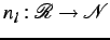
Let
 denote
a fixed arithmetic lattice
supporting digital images
denote
a fixed arithmetic lattice
supporting digital images
 where
where  is a finite set of grey levels, where measure the intensity of a pixel.
Let
is a finite set of grey levels, where measure the intensity of a pixel.
Let  and
and  be two noisy images of a stereo pair to be matched and let
 be their hidden ``cyclopean" noiseless template, or prototype, such
that each its pixel
be their hidden ``cyclopean" noiseless template, or prototype, such
that each its pixel  relates to the corresponding pixels
 and
and  in
in  and
and  ,
respectively. Let
,
respectively. Let
 denote image noise for an individual pixel.
In line with the discussion of robustness to
noise by Leclercq and
Morris [70,71], the
signal-to-noise ratio (SNR)
of an image is defined as the ratio of the mean pixel value to the
standard deviation of the pixel values. A closely related
``contrast-to-noise ratio" (CNR) replaces the mean pixel value with
the mean absolute signal differences between the neighbouring
pixels. Visually, the more grainy an image, the lower the SNR. The CNR
is
measured frequently by calculating the absolute difference in
intensity between an area of interest (a particular object) and the
background surrounding the object. The difference is divided by the
standard deviation of the background signals that indicates the
variability of the background.
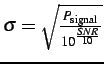
The level of the additive white Gaussian
noise is defined by:
where

denotes the
power. An SNR of 0 dB implies equal
signal and noise powers; increasing an SNR by 3 dB doubles the
signal's power. For a discrete image, in which

is the
intensity of a pixel

,
the power is specified as
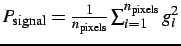
.
If the noise is assumed to have a centred Gaussian distribution,
,
the power of the noise is:

.
To produce an image with power,

, and
desired SNR, white noise was added with standard deviation:
 3.1
3.1.
Figure
![[*]](crossref.png)
shows images with increasing
levels of noise. At

dB, the
image contains little
valid information. To place this noise definition in context,
observe that

dB produces
images which appear
similar to the ``perfect" one, although this SNR implies noise with

in a range
of

and
therefore noise
values of

%
of signal values with a mean intensity of

. This represents a large
error,

%
(i.e. 6 in 153).
Thus a good camera in a well-lighted scene would produce SNR's of 40
dB or more.
Figure:
Image with varying SNR's
![\includegraphics[scale=0.15]{Corridor-P-R.eps}](img260.png) |
![\includegraphics[scale=0.15]{Corridor-P-R-N_AWGN-60dB.eps}](img261.png) |
![\includegraphics[scale=0.15]{Corridor-P-R-N_AWGN-48dB.eps}](img262.png) |
![\includegraphics[scale=0.15]{Corridor-P-R-N_AWGN-36dB.eps}](img263.png) |
| No noise |
SNR = 60 dB |
SNR = 48 dB |
SNR = 36 dB |
![\includegraphics[scale=0.15]{Corridor-P-R-N_AWGN-24dB.eps}](img264.png) |
![\includegraphics[scale=0.15]{Corridor-P-R-N_AWGN-12dB.eps}](img265.png) |
![\includegraphics[scale=0.15]{Corridor-P-R-N_AWGN-0dB.eps}](img266.png) |
![\includegraphics[scale=0.15]{Corridor-P-R-N_AWGN--12dB.eps}](img267.png) |
| SNR = 24 dB |
SNR = 12 dB |
SNR = 0 dB |
SNR = -12 dB |
|
Image noise arises from the following
sources [16]:
- Group 1: Signal noise
- Group 2: Geometric sources
- Group 3: Electronic sources
- Group 4: Optical sources
Group 1 noise arises from
electromagnetic interference (e.g.
cross-talk), quantum behaviour of electronic devices (e.g. resistor
shot-noise) and quantisation noise introduced when a real-valued
analogue signal is digitised. Noise of Group 2 is caused by
discrete
pixel sensors with finite area, partial occlusions of 3D objects
viewed from different directions and perspective distortions.
Electronic sources (Group 3) include intensity sensitivity
variations between cameras (e.g. different optical or electronic
gain settings) and different ``dark noise" levels. Noise of
Group 4
results from non-uniform scattering (non-Lambertian surfaces),
reflections and specular highlights, angle dependent colour
scattering (``grating" effects) and lighting variation due to
different view angles.
Sources in Group 1 are common to
almost all electronic measurement
equipment and introduce random perturbations in measured
intensities. Group 2 sources arise from the internal structure
of
digital cameras themselves and the stereo system configuration. Some
configurations avoid Group 3 noise by using a single camera on
a
translation base or a moving scene (e.g. object on a rotation
stage). However, this noise is unavoidable in any two-camera stereo
set-up. The physical separation of the two cameras results in
different viewing angles and produces the last group of problems
(Group 4). Most matching algorithms make the unrealistic
assumptions
that all the observed surfaces are perfect Lambertian scatterers.
Figure:
`Corridor': Noise in ``ideally matching" pixels (scan line 152/256). In
right image, the grey-level intensity plots across the left
image (top), the
actual depth profile obtained from ground truth maps (bottom)
and
differences between the corresponding pixels in left and right
images (centre)
|
|
Figure:
`Tsukuba': Noise in ``ideally matching" pixels (scan line 173/288).
|
|
Most matching algorithms make very simple
assumptions about these
noise sources, particularly, about the random sources (Group 1
noise). Typically, the absolute or squared intensity difference is
used as a dissimilarity measure so that sum of absolute differences
(SAD) or sum of square differences (SSD) between corresponding
pixels act as a dissimilarity measure for a stereo pair. Common
techniques which minimise the SAD or SSD under 2D constraints
imposed by anticipated occlusions and surface smoothness include
graph
minimum-cut [1,51,45,72,69]
and belief propagation algorithms [73,53,52].
Calculating a correlation over a moving window attempts to allow for
Group 3 noise and lighting variations of Group 4
noise [26,74]. Dynamic
programming (DP) algorithms
finding a best ``path" through the disparity space use mostly the
same SAD or SSD matching criteria [37,33,32].
Symmetric dynamic programming stereo (SDPS) algorithm [68,40] also allows
for limited offset and contrast noise being independent for each
conjugate pair of epipolar scan-lines.
Conventional stereo matching algorithms
invariably start by seeking
a ''best'' match, considering only a single pixel, a
small 1D
sequence of pixels or a small 2D pixel neighbourhood. This best
match appears in different forms: in simple window matching
algorithms, it directly appears that the best matching window is
selected and others are rejected. The window size is chosen as a
compromise between noise reduction and feature smoothing. In DP algorithms, a best path in a graph representing possible
depth profiles is chosen minimizing total matching errors over a
sequence of pixels. In 2D energy minimization approaches (e.g. graph
min-cut or belief propagation), the lowest ``energy" is chosen; the
energy terms describing either an intensity mismatch or differences
for two adjacent pixels. In the presence of so many ``noise"
sources, searching for a single minimum (or maximum for correlation
functions) is inherently unsatisfactory and leads to large numbers
of reconstruction errors due to the rejection of ``close" matches
which are actually correct, but perturbed by image or system noise.
Matching problems induced by actual image
noise are illustrated
below on (a) the synthetic `Corridor' [75] and (b) the
real `Tsukuba' [76]
stereo image sets. Corresponding pixels were determined by using
ground truth data, so one might expect a small mismatch arising only
from signal (Group 1) noise. The `Corridor' image was produced
by
ray-tracing and are free of signal (Group 1) and electronic
(Group 3) noise. The actual mismatches are very much larger
and
usually associated with edge of individual objects in the image.
However, some edges present a very small mismatch - a level
associated with signal noise alone. The presence of significant
numbers of intensity differences in this image is entirely due to
geometric (Group 2) and optical (Group 4) noise and
emphasises the
difficulty in selecting corresponding points.
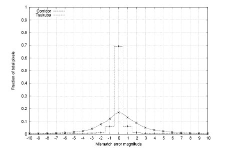
Figure
shows the distribution of noise for the
full images: note that the signal-noise-free `Corridor' image shows
only 70% close matches, i.e. 30% of pixels do not match because of
geometric and optical problems! Moreover, there is only one small
occlusion in Figure - the most ``obvious"
of the geometric (Group 2) noise sources - a small region
around
position 230 in the scan line.
Figure:
Empirical noise distributions: for clarity, `Corridor' is shown as a
histogram; `Tsukuba' as a smooth curve. The similar empirical noise
distributions for other stereo pairs are given in Chapter 4.
|
|
Recently a framework for searching for a
minimal photo-consistent
hull containing no spatial elements (voxels) resulting in dissimilar
corresponding points was introduced to reconstruct a 3D surface from
multiple images [77].
Also, humans tend to analyse a
scene by strokes - the eye's focus browsing from low to high
frequency regions, from sharp points to smooth areas and vice versa
rather than scanning line-by-line [78]. Starting
with
these ideas, a novel framework for concurrent binocular stereo
reconstruction is introduced and named ``Noise-driven Concurrent
Stereo Matching" (NCSM), leveraging advantages and reducing
disadvantages of previous methods.
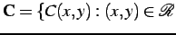
As each typical stereo pair contains many
admissible matches,
``best" matching algorithms may make many incorrect decisions. To
counter this, NCSM separates image matching from a subsequent search
for surfaces. It considers all likely matching volumes instead of
singleton local best matches and exploits local surface constraints
rather than global continuity ones. NCSM has three main features:
- The noise is estimated at every point.
- Corresponding volumes are found by
image-to-image matching at each fixed depth, or disparity value; this
allows photometric distortions of images to be taken into account.
- 3D reconstruction proceeds from
foreground to background surfaces in order to account for occlusions
and enlarges corresponding background volumes at the expense of
occluded portions;
an additional colouring continuity criterion is then used to select
most appropriate surfaces.
Because the well-known `Tsukuba' image pair
(
Figure ) is a real scene with several
distinct depth (disparity) layers (termed `d-slices'), it was used
to illustrate each stage in the NCSM framework.
Figure:
`Tsukuba' stereo pair:
First row - colour left and right images; second row - greyscale
and colour coded true disparity map; last two rows - selected
`slices' of the ideal disparity map showing which regions appear at
the indicated disparity.
|
|
NCSM first matches image pixels using a
signal model to estimate
random signal noise which is independent in both images and can be
spatially variant. The model takes into account possible global or
local contrast and offset deviations between the corresponding image
areas. In contrast to more conventional approaches, rather than
immediately trying to find the single optical surface or its minimal
visual hull, NCSM first delimits all 3D volumes which are
reconstruction candidates, i.e. contain the candidate 3D points
ensuring an admissible (or good) match to within the noise model.
In the second stage, NCSM attempts to find
surfaces fitting the
candidate volumes using only smoothness and visibility constraints
that rank the surfaces according to their appropriateness for
human visual perception. The fundamentally ill-posed nature
of the
problem makes discovering the true surface an unrealistic goal.
Thus, a more practical goal is set to select from possible
candidates a surface that closely resembles the choice that a human
observer would make.
In the final stage, one or more surfaces are
selected and possible
partial occlusions of the chosen surfaces are analysed. In this
study, surfaces were stratified into foreground versus background
and refining the occluded background after eliminating the
foregrounds; Other strategies for this step could be explored in
future work. By retaining all likely solutions for a given set of
images, the imposition of constraints which are not always
physically realistic is delayed until the final stage where they
guide choices of possible solutions. Figure
illustrates the work flow of NCSM.
Figure:
Data flow diagram for NCSM
|
|
Signal similarity models for matching need
to account for changes in
surface reflection as the scattering angle changes and for many
other potential noise sources. However, most of the conventional
stereo matching algorithms, including the best-performing belief
propagation and graph minimum-cut ones, use first-order similarity
criteria such as SAD or SSD for all binocularly visible surface
points. The underlying signal model assumes equal corresponding
signals distorted by an additive independent noise with symmetric
zero-centred distribution. This simplification is justified only for
a few stereo pairs typically used by researchers for testing stereo
algorithms, for example the Middlebury data set [4].
However, it is invalid in many practical applications, which may
need to process, for example, aerial or ground image pairs of
terrain collected at different times under changing illumination and
image acquisition conditions. To be realistic, similarity models
must at least account for global or local contrast and offset signal
distortions [67,68].
This section presents two possible approaches to noise estimation at
the first stage of NCSM . The first approach, referred as
NCSM with SDPS noise estimation (NCSM-SDPS), accounts for contrast and offset distortions along
conjugate epipolar lines but not for inter-dependence of these
distortions between lines. The second approach, referred as
NCSM with iterative noise estimation (NCSM-ITER), is more realistic because it assumes contrast and offset
distortions are independent for scene points at the same depth
(disparity) level. In the discussion following, `profile' refers to
a depth for disparity profile which relates to a pair of
corresponding epipolar lines.
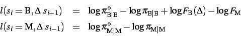
Basically, SDPS reconstructs profiles of a stereo pair by maximising
the log-likelihood ratio that compares the corresponding signals
along the profile to a purely random profile. Regularisation with
respect to partial occlusions is based on Markov chain models of
epipolar profiles and image signals along a
profile [
68,
40]. The models
distinguishes between
binocularly and monocularly visible points. Non-uniform relative
photometric distortions of images are taken into account by
adaptation of the corresponding signals along each profile.
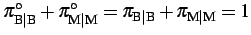
The Markov model of profile is controlled by
two probabilities of
transition from a current binocularly or monocularly visible point to the adjacent BVP or MVP, respectively. Let these
probabilities be denoted,
 and
and
 ,
for the profile reconstructed
from a given stereo pair and
,
for the profile reconstructed
from a given stereo pair and
 and
and
 for
the purely random profile,
respectively. For simplicity, only single-parameter geometric models
of the profiles,
for
the purely random profile,
respectively. For simplicity, only single-parameter geometric models
of the profiles,
 ,
are considered below.
,
are considered below.
Conditional signal probabilities depend on
the visibility of a
profile point. For the BVPs, the probability,
 ,
steadily decreases with the increasing devialtion
,
steadily decreases with the increasing devialtion  between
signals. The signal intensities for MVPs are equiprobable:
between
signals. The signal intensities for MVPs are equiprobable:
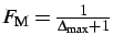 where
where  is the
maximum deviation. Because of the adaptation, the assumed
probability model for the BVPs reinforces the zero-deviation
probability,
is the
maximum deviation. Because of the adaptation, the assumed
probability model for the BVPs reinforces the zero-deviation
probability,  ,
with respect to all other deviations:
,
with respect to all other deviations:
 |
(3.2.1) |
Here,

is the scaling factor and

is the threshold
for omitting zero probabilities in the log-likelihood ratios (in our
experiments

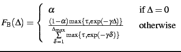
). Every
profile,

,
is
specified by its starting BVP,

, and a chain of the
visibility states,

,
of successive points

. The
desired profile,

, maximises
the
cumulative log-likelihood ratio that relates the probability of the
profile yielding signal correspondences to the probability of a
purely random profile with equiprobable signals for both the BVPs
and MVPs [
40]:
 |
(3.2.2) |
where

is the point-wise
log-likelihood ratio measuring the similarity of corresponding
signals for the transition between adjacent visibility states,

and
:
 |
(3.2.3) |
The transition probabilities for the Markov profile models act as
regularising parameters.
Because SDPS accounts for continuity,
smoothness and visibility
constraints along profile, it results in explicit estimates of BVPs
and MVPs in the reconstructed surface. Generally, a prior random
field model of noise can be specified to formulate the noise
estimation problem as a Bayesian inference with due account of the
BVPs and MVPs. Thus, SDPS-based noise estimation discriminates
between the effects of a small subset of occluded pixels,  ,
and the effects of an additive imaging noise,
,
and the effects of an additive imaging noise,  ,
interpolated over the entire image. Consequently, the SDPS-estimated
noise allows us to approximately determine which matches are
admissible. Obviously, images with finer texture need more robust
noise estimation models taking account of sub-pixel quantisation
errors [79].
,
interpolated over the entire image. Consequently, the SDPS-estimated
noise allows us to approximately determine which matches are
admissible. Obviously, images with finer texture need more robust
noise estimation models taking account of sub-pixel quantisation
errors [79].
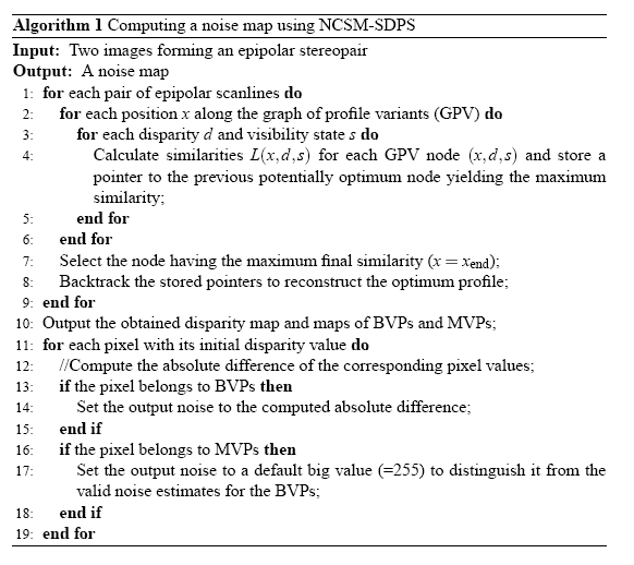
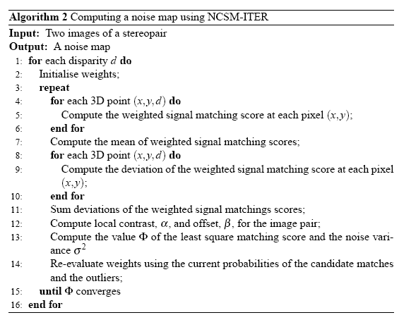
Algorithm
describes noise estimation using SDPS
in pseudo-code. Figure presents
outputs of NCSM-SDPS: first, the disparity, MVP and BVP maps are
obtained by SDPS; then, the noise map containing absolute
differences of corresponding pairs is computed.
The estimated noise map allows us to outline
candidate 3D volumes by
setting upper bounds for noise. Let
 be a map of pixel-wise upper bounds for the admissible
noise on the left image obtained by comparing empirical probability
distributions of noise of individual pixels and outliers. A
candidate volume,
be a map of pixel-wise upper bounds for the admissible
noise on the left image obtained by comparing empirical probability
distributions of noise of individual pixels and outliers. A
candidate volume,  ,
for a pixel,
,
for a pixel,  in the left
image, is a collection of disparities such that the noise estimate
for them is bounded by
in the left
image, is a collection of disparities such that the noise estimate
for them is bounded by  :
:
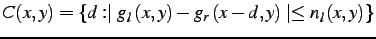 |
(3.2.4) |
where
is the
absolute difference of the corresponding signals for
the disparity, BVP and MVP maps obtained by SDPS.
Figure:
Outputs of SDPS for the `Tsukuba' stereo pair: (a) the
initial disparity map; (b) the MVPs map; (c) the BVPs
map, and
(d) the scaled noise map. Note: in (b) and (c), the black
points
indicate MVPs and BVPs, respectively.
|
|
To demonstrate the first stage of NCSM-SDPS,
Figure
presents slices of the
candidate volumes,
,
at
constant disparity levels,

,
(the slices are called
-slices
below). Black points in the
-slice
indicate candidate 3D points
producing ``matches" defined by Eq.
.
Figure:
-slices
of the candidate volumes for the `Tsukuba'
stereo pair found by NCSM-SDPS
|
|
NCSM-SDPS assumes independent contrast and
offset distortions along
each conjugate pair of epipolar lines. More adequate noise
estimation should consider interdependent global or local contrast
and offset distortions which are more likely for stereo images due
to different surface albedo in different directions.
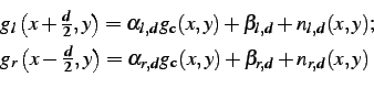
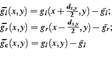
Compared to conventional assumptions
about image noise, in NCSM-ITER, a more general noise model allows
gain offset and noise contributions to vary spatially. Since
different disparity slices relate to different scene regions, this
effectively means that different values for
and

and

are allowed for each image and in each d-slice:
 |
(3.2.5) |
where the noise terms

contains two components: (
i) a
centred Gaussian or more general symmetric noise with zero math
expectation
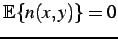
for corresponding areas
(candidate matches) in the images and (
ii)
outliers having
uniform distribution of their squared values over the range of
signal differences. The model is more restrictive than SDPS in that
the contrast and offset variations are constant for the whole
template, but it is more general in that it accounts for possible
outliers.
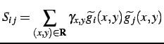
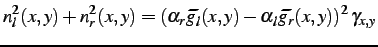
The basic idea is that the noise slowly
changes across the lattice
but is relatively small in the matching areas. The outliers have
large signal differences and change arbitrarily, and the images may
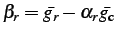
differ in local contrast, , and offset, ,
characteristics so that the simple signal differences used almost
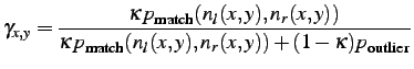
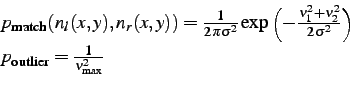
universally as matching scores do not work. A disparity level, ,
let a special soft label, or weight,
![$ \gamma_{x,y}\in[0,1]$](img355.png) ,
indicate the probability that a pixel pair
belongs to true candidate matches rather than to outliers in each
image. The probability decreases monotonously with the absolute
signal difference. Let the noise have the same unknown standard
deviation
,
indicate the probability that a pixel pair
belongs to true candidate matches rather than to outliers in each
image. The probability decreases monotonously with the absolute
signal difference. Let the noise have the same unknown standard
deviation  ,
then the least square matching score is
obtained using the maximum likelihood estimates for the hidden
parameters
,
then the least square matching score is
obtained using the maximum likelihood estimates for the hidden
parameters
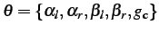 of the ``pure
noise" - outlier models:
of the ``pure
noise" - outlier models:
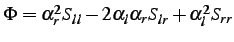
![\begin{displaymath}\begin{array}{lll} \Phi & = & \min_{\boldmath {\theta}}\sum\... ...- \alpha_2 g_\mathrm{c}(x,y) - \beta_2 \right)^2] \end{array}\end{displaymath}](img358.png) |
(3.2.6) |
Local optimisation in Eq. (
) proceeds iteratively:
the weights are evaluated again after the matching score is found
with the current weights using a simple rule that follows from the
assumed ``pure noise"-outlier model which specifies how these two
classes are responsible for the evaluated noise:
 |
(3.2.7) |
Here,

denotes a prior probability of the candidate
matches and

and

are the current joint probability densities of the two noise values
for the pixel pair being the candidate match and of the outliers,
e.g. the joint Gaussian density where the variance relates to the
matching score,

,
and the uniform density, respectively:
 |
(3.2.8) |
Taking derivatives of
the matching score with respect to the unknown parameters leads to
the following system of equations, given fixed weights:
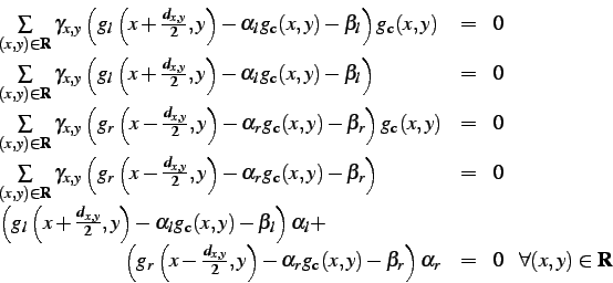 |
(3.2.9) |
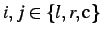
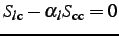
It follows that
 ;
;
 ,
and
,
and

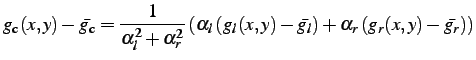 |
(3.2.10) |
where bars denote weighted mean signals:
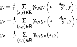 |
(3.2.11) |
where
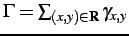
.
Let
Centred signals are denoted with tildes:
 |
(3.2.12) |
and the sums of their products are denoted as:
 |
(3.2.13) |
where
.
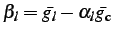
Then the relationships,
,
and
where
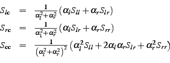 |
(3.2.14) |
allow us to introduce a constraint,
,
and
obtain
.
Therefore,
![\begin{displaymath}\begin{array}{l} \alpha_1^2 = \frac{1}{2}\left( 1 + \frac{S... ...2})^2 + 4S_{12}^2 \right]^{\frac{1}{2}}} \right) \end{array}\end{displaymath}](img380.png) |
(3.2.15) |
and
.
The estimated noise variance is

,
and the squared joint intensity noise is as
follows:
 |
(3.2.16) |
The latter two relationships allow for iterative re-evaluation of
the current weights. Iteration terminates when the matching score
changes by less than a threshold. The weights outline regions for
candidate matching, e.g.

,
where

is a reasonable threshold in the range
![$ [0.5, 1]$](img386.png)
.
Noise estimation using the iterative
approach, NCSM-ITER, is
outlined by Algorithm in pseudo-code. The noise
map is obtained iteratively, by re-evaluating the weights after the
matching score is found using the current weights.
To demonstrate the first stage of NCSM-ITER,
Figure
presents
-maps
obtained for

slices
either after ten iterations or convergence
(no significant change in
)
if it occurred earlier.
values in
![$ [0.0, 1.0]$](img389.png)
converted
to a
![$ [0, 255]$](img390.png)
grey scale
for visualisation.
values near 1 (white points) respresent
the lower noise. Noise maps computed for the
slices with
Eq. (
)
are presented in
Figure
. Here, white regions
correspond to the higher noise.
Figure
shows the -slices
of the
candidate volumes, ,
where black points indicate candidate
``matches". These results differ visually from the candidate volumes
derived with NCSM-SDPS. However, the candidate volumes for
NCSM-ITER are equally suitable for the subsequent surface fitting
stage. For instance, the lamp appears in the 14th slice, because, in
both cases, the slice with the largest number of good matches (i.e.
black points) compared to other disparity levels.
Figure:
-maps
for -slices for
the `Tsukuba' stereo
pair obtained by NCSM-ITER.
|
|
Figure:
Noise maps for -slices
for the `Tsukuba' stereo pair
obtained by NCSM-ITER.
|
|
Figure:
-slices
of the candidate volumes for the `Tsukuba'
stereo pair obtained by NCSM-ITER.
|
|
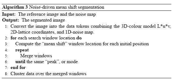
To simplify 3D surface reconstruction, it is assumed that each
surface patch of uniform colouring has a single unknown disparity.
Based on estimated noise, each stereo image can be segmented onto
uniform regions depicting uniformly coloured spatial patches. For
such noise-driven segmentation of colour stereo images, the mean
shift algorithm [
65]
based on colour-position
clustering in a 5D feature space, constructed from an L*u*v colour
space triple and a 2D lattice coordinates was used. The Euclidean
distance in the colour space closely approximates visual colour
discrimination, so that the admissible matches can be specified by
simple thresholding. Consequently, the map of admissible noise
bounds after estimating the noise is considered as the extra sixth
dimension.
During segmentation, an image is filtered
first by replacing the
colour in each pixel with the colour component of the closest 5D
mode the pixel relates to in the feature space. This filter
preserves signal discontinuities. Then, the attraction domains of
each mode in the colour space are iteratively fused until the
segmentation becomes stable, and all the pixels in each region are
set to the mean colour value. The noise-driven segmentation
algorithm uses a modified mean-shift method
that combines the noise in each position with the 3D-colour space
and 2D coordinates in order to convert the reference image with
noise into the mean-shift data tokens.
Figure
presents the noise map derived by
NCSM-SDPS and results of segmenting the `Tsukuba' image with the
noise-driven and conventional mean-shift algorithms.
Figure:
(a) NCSM-SDPS noise map scaled to for visualisation; white
regions mainly represent mainly occlusions (high noise); (b)
noise-driven segmentation.
![\includegraphics[width=1.7in]{tsukuba_symm_noise_l.eps}](img440.png) |
![\includegraphics[width=1.7in]{tsukuba_noise_segm_l.eps}](img441.png) |
| (a) |
(b) |
|
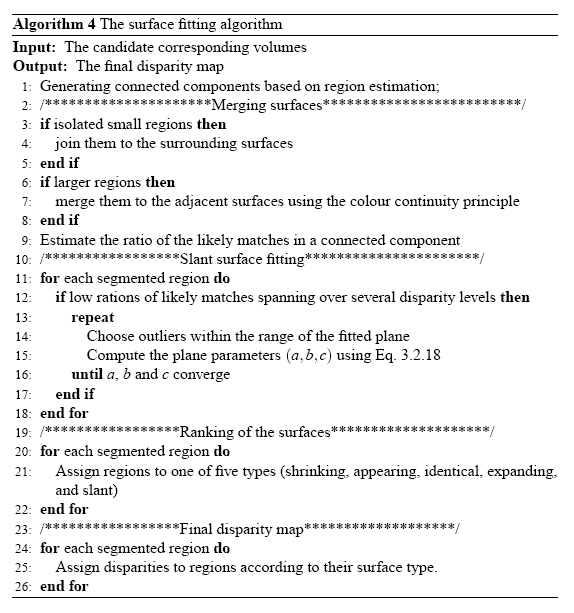
After all the likely matching pixels at each disparity level are
merged in the reference image into regions (or suppressed) by the
noise-driven mean shift algorithm and the candidate volumes are
formed, surfaces are fitted in these steps:
- Cnnected components are generated based
on region estimation.
- Surfaces are merged: (a) isolated small
regions (typically, segments representing occluded parts of a scene)
are joined to the surrounding surface and (b) larger regions are joined
to the surfaces using the same ``colour continuity" principle as the
colour mean shift segmentation.
- The ratio of likely matches in a
connected component versus the same area at any given -slice is
estimated.
- Slanted surfaces for the low ratios of
good matches (the slanted surface propagates over multiple disparity
levels).
- Connected components borders are further
processed by intra- and inter-region statistical analysis.
During the third step, for each connected
component or region, a
distribution of the count of good matches with that region versus
disparity is generated. The maximum of this distribution is the -slice
which will survive as a potential candidate for the
disparity, .
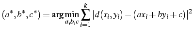
Segmented regions with low ratios of good matches
over a number of adjacent disparity levels are considered as slant
planar surfaces,  ,
with parameters
,
with parameters  ,
,
 ,
and
,
and  estimated
by least squares:
estimated
by least squares:
 |
(3.2.17) |
where

is the
number of pixels in the related regions so that
![$\displaystyle \left[ \begin{array}{l} a^\ast \\ b^\ast \\ c^\ast \end{arra... ...k}y_{i}d(x_{i},y_i) \\ \sum\limits_{i=1}^{k}d(x_{i},y_i) \end{array} \right]$](img447.png) |
(3.2.18) |
To rank surface variants in the
corresponding volumes in accord with
visual perception, a heuristic preference criterion based on surface
planarity, area, and its local expansion or shrinkage in the
adjacent -slices
was used. Every connected component was
dynamically assigned to one of the following five classes based on
its behaviour in the -slices:
- ``shrinking" from slice,
 , to slice, ,
- ``appearing" in the current -slice,
- ``not changing" in slices, and ,
- ``expanding" from slice, , to slice, ,
- ``slanting" from slice,
 , to slice,
  .
.
At any given disparity, these labels express the likelihood of
``good matching" and indicate the expansion or contraction of the
candidate volumes in the

space. This surface fitting
algorithm
processes the connected components in a
reference image by intra- and inter-region statistical analysis and
handles both horizontal (with constant disparity
) and
slanted
planar surfaces.
Figures
and
present
-slices of
surface patches for the `Tsukuba' stereo pair that survived after
the surface fitting applied to the candidate volumes estimated by
NCSM-SDPS and NCSM-ITER, respectively. The final disparity
maps (DPM) in Figure
show that
NCSM-SDPS and NCSM-ITER produce quite similar results in this
particular case. However, as shown in the next chapter, these
matching algorithms have different behaviour with the different
levels of noise.
Figure:
Surface patches in the -slices
for the `Tsukuba'
stereo pair that survived after surface fitting to candidate
volumes obtained by NCSM-SDPS.
|
|
Figure:
Surface patches in the -slices
for the `Tsukuba'
stereo pair that survived after surface fitting to candidate
volumes obtained by NCSM-ITER.
|
|
Figure:
Final disparity map for NCSM-SDPS (left) and NCSM-ITER (right).
|
|
In this Chapter, first an analysis of image
noise was presented with
multiple noise sources including random variations of sensitivity of
optical sensors, non-Lambertian surface reflection, specific impacts
of geometry of stereo observation (e.g. occlusions), etc. Although
stereo matching criteria and strategies obviously depend on all the
noise components, most conventional stereo algorithms use only a
very simple and thus unrealistic models of random pixel noise.
A new alternative approach to 3D stereo
reconstruction based on a
layered model of an observed 3D scene, called Noise-driven
Concurrent Stereo Matching (NCSM) was developed in the second
part
of this Chapter. This framework reduces drawbacks of more
conventional previous ones due to more general image noise models
and less restrictive matching goals. The framework separates 3D
reconstruction into two independent stages:
- The image
noise estimation outlines spatial candidate volumes being equivalent
from the standpoint of image matching under the noise. Two schemes
for noise estimation, NCSM-SDPS and NCSM-ITER, were used in this
stage. The NCSM-SDPS algorithm takes account of possible contrast
and offset distortions combined with independent intensity random
deviations and occlusions along epipolar lines and the second
algorithm, NCSM-ITER, involves a more realistic spatial noise model
with uniform contrast and offset distortions for all the scene
points at the same depth level, the distortions being independent on
the different levels
- The selection of one or more
surfaces is to fit candidate volumes with due account of partial
occlusions of background objects with foreground ones.
This framework circumvents the ``best match"
or ``closest
similarity" criteria exploited in almost all existing matching
strategies in favour of a likely match criterion based on a local
model of signal noise.
![\includegraphics[width=5.0cm]{Corridor-P-L.eps}](img268.png)
![\includegraphics[width=7.0cm]{Corr152NoiseR.eps}](img269.png)
![\includegraphics[width=5.5cm]{tsukuba-l-173marked.eps}](img270.png)
![\includegraphics[width=6.5cm]{Tsukuba173NoiseRA.eps}](img271.png)
![\includegraphics[width=6cm]{mb/tsukuba/tsukuba-l.ppm.eps}](img273.png)
![\includegraphics[width=6cm]{mb/tsukuba/tsukuba-r.ppm.eps}](img274.png)
![\includegraphics[width=6cm]{mb/tsukuba/tsukuba-disp.pgm.eps}](img275.png)
![\includegraphics[width=6cm]{mb/tsukuba/tsukuba-disp-c.ppm.eps}](img276.png)
![\includegraphics[width=3cm]{mb/tsukuba/tsukuba_ideasurfaces_at_disp5.pgm.eps}](img284.png)
![\includegraphics[width=3cm]{mb/tsukuba/tsukuba_ideasurfaces_at_disp6.pgm.eps}](img285.png)
![\includegraphics[width=3cm]{mb/tsukuba/tsukuba_ideasurfaces_at_disp7.pgm.eps}](img286.png)
![\includegraphics[width=3cm]{mb/tsukuba/tsukuba_ideasurfaces_at_disp8.pgm.eps}](img287.png)
![\includegraphics[width=3cm]{mb/tsukuba/tsukuba_ideasurfaces_at_disp10.pgm.eps}](img288.png)
![\includegraphics[width=3cm]{mb/tsukuba/tsukuba_ideasurfaces_at_disp11.pgm.eps}](img289.png)
![\includegraphics[width=3cm]{mb/tsukuba/tsukuba_ideasurfaces_at_disp14.pgm.eps}](img290.png)
![\includegraphics[width=3.0in]{ncsm-1.eps}](img291.png)
![\includegraphics[width=3.3cm]{mb/tsukuba/tsukuba-left-sdps-dpm.pgm.eps}](img321.png)
![\includegraphics[width=3.3cm]{mb/tsukuba/tsukuba-left-sdps-bvp.pgm.eps}](img322.png)
![\includegraphics[width=3.3cm]{mb/tsukuba/tsukuba-left-sdps-mvp.pgm.eps}](img323.png)
![\includegraphics[width=3.3cm]{mb/tsukuba/tsukuba-left-sdps-noise-s6.pgm.eps}](img324.png)
![\includegraphics[width=3.3cm]{mb/tsukuba/sdps/10-confidenceMap_at_0.pgm.eps}](img336.png)
![\includegraphics[width=3.3cm]{mb/tsukuba/sdps/10-confidenceMap_at_1.pgm.eps}](img337.png)
![\includegraphics[width=3.3cm]{mb/tsukuba/sdps/10-confidenceMap_at_2.pgm.eps}](img338.png)
![\includegraphics[width=3.3cm]{mb/tsukuba/sdps/10-confidenceMap_at_3.pgm.eps}](img339.png)
![\includegraphics[width=3.3cm]{mb/tsukuba/sdps/10-confidenceMap_at_4.pgm.eps}](img340.png)
![\includegraphics[width=3.3cm]{mb/tsukuba/sdps/10-confidenceMap_at_5.pgm.eps}](img341.png)
![\includegraphics[width=3.3cm]{mb/tsukuba/sdps/10-confidenceMap_at_6.pgm.eps}](img342.png)
![\includegraphics[width=3.3cm]{mb/tsukuba/sdps/10-confidenceMap_at_7.pgm.eps}](img343.png)
![\includegraphics[width=3.3cm]{mb/tsukuba/sdps/10-confidenceMap_at_8.pgm.eps}](img344.png)
![\includegraphics[width=3.3cm]{mb/tsukuba/sdps/10-confidenceMap_at_9.pgm.eps}](img345.png)
![\includegraphics[width=3.3cm]{mb/tsukuba/sdps/10-confidenceMap_at_10.pgm.eps}](img346.png)
![\includegraphics[width=3.3cm]{mb/tsukuba/sdps/10-confidenceMap_at_11.pgm.eps}](img347.png)
![\includegraphics[width=3.3cm]{mb/tsukuba/sdps/10-confidenceMap_at_12.pgm.eps}](img348.png)
![\includegraphics[width=3.3cm]{mb/tsukuba/sdps/10-confidenceMap_at_13.pgm.eps}](img349.png)
![\includegraphics[width=3.3cm]{mb/tsukuba/sdps/10-confidenceMap_at_14.pgm.eps}](img350.png)
![\includegraphics[width=3.3cm]{mb/tsukuba/sdps/10-confidenceMap_at_15.pgm.eps}](img351.png)
![\includegraphics[width=3.3cm]{mb/tsukuba/iter/11-GammaMap_at_0.pgm.eps}](img391.png)
![\includegraphics[width=3.3cm]{mb/tsukuba/iter/11-GammaMap_at_1.pgm.eps}](img392.png)
![\includegraphics[width=3.3cm]{mb/tsukuba/iter/11-GammaMap_at_2.pgm.eps}](img393.png)
![\includegraphics[width=3.3cm]{mb/tsukuba/iter/11-GammaMap_at_3.pgm.eps}](img394.png)
![\includegraphics[width=3.3cm]{mb/tsukuba/iter/11-GammaMap_at_4.pgm.eps}](img395.png)
![\includegraphics[width=3.3cm]{mb/tsukuba/iter/11-GammaMap_at_5.pgm.eps}](img396.png)
![\includegraphics[width=3.3cm]{mb/tsukuba/iter/11-GammaMap_at_6.pgm.eps}](img397.png)
![\includegraphics[width=3.3cm]{mb/tsukuba/iter/11-GammaMap_at_7.pgm.eps}](img398.png)
![\includegraphics[width=3.3cm]{mb/tsukuba/iter/11-GammaMap_at_8.pgm.eps}](img399.png)
![\includegraphics[width=3.3cm]{mb/tsukuba/iter/11-GammaMap_at_9.pgm.eps}](img400.png)
![\includegraphics[width=3.3cm]{mb/tsukuba/iter/11-GammaMap_at_10.pgm.eps}](img401.png)
![\includegraphics[width=3.3cm]{mb/tsukuba/iter/11-GammaMap_at_11.pgm.eps}](img402.png)
![\includegraphics[width=3.3cm]{mb/tsukuba/iter/11-GammaMap_at_12.pgm.eps}](img403.png)
![\includegraphics[width=3.3cm]{mb/tsukuba/iter/11-GammaMap_at_13.pgm.eps}](img404.png)
![\includegraphics[width=3.3cm]{mb/tsukuba/iter/11-GammaMap_at_14.pgm.eps}](img405.png)
![\includegraphics[width=3.3cm]{mb/tsukuba/iter/11-GammaMap_at_15.pgm.eps}](img406.png)
![\includegraphics[width=3.3cm]{mb/tsukuba/iter/11-NoiseMap_at_0.pgm.eps}](img407.png)
![\includegraphics[width=3.3cm]{mb/tsukuba/iter/11-NoiseMap_at_1.pgm.eps}](img408.png)
![\includegraphics[width=3.3cm]{mb/tsukuba/iter/11-NoiseMap_at_2.pgm.eps}](img409.png)
![\includegraphics[width=3.3cm]{mb/tsukuba/iter/11-NoiseMap_at_3.pgm.eps}](img410.png)
![\includegraphics[width=3.3cm]{mb/tsukuba/iter/11-NoiseMap_at_4.pgm.eps}](img411.png)
![\includegraphics[width=3.3cm]{mb/tsukuba/iter/11-NoiseMap_at_5.pgm.eps}](img412.png)
![\includegraphics[width=3.3cm]{mb/tsukuba/iter/11-NoiseMap_at_6.pgm.eps}](img413.png)
![\includegraphics[width=3.3cm]{mb/tsukuba/iter/11-NoiseMap_at_7.pgm.eps}](img414.png)
![\includegraphics[width=3.3cm]{mb/tsukuba/iter/11-NoiseMap_at_8.pgm.eps}](img415.png)
![\includegraphics[width=3.3cm]{mb/tsukuba/iter/11-NoiseMap_at_9.pgm.eps}](img416.png)
![\includegraphics[width=3.3cm]{mb/tsukuba/iter/11-NoiseMap_at_10.pgm.eps}](img417.png)
![\includegraphics[width=3.3cm]{mb/tsukuba/iter/11-NoiseMap_at_11.pgm.eps}](img418.png)
![\includegraphics[width=3.3cm]{mb/tsukuba/iter/11-NoiseMap_at_12.pgm.eps}](img419.png)
![\includegraphics[width=3.3cm]{mb/tsukuba/iter/11-NoiseMap_at_13.pgm.eps}](img420.png)
![\includegraphics[width=3.3cm]{mb/tsukuba/iter/11-NoiseMap_at_14.pgm.eps}](img421.png)
![\includegraphics[width=3.3cm]{mb/tsukuba/iter/11-NoiseMap_at_15.pgm.eps}](img422.png)
![\includegraphics[width=3.3cm]{mb/tsukuba/iter/11-confidenceMap_at_0.pgm.eps}](img423.png)
![\includegraphics[width=3.3cm]{mb/tsukuba/iter/11-confidenceMap_at_1.pgm.eps}](img424.png)
![\includegraphics[width=3.3cm]{mb/tsukuba/iter/11-confidenceMap_at_2.pgm.eps}](img425.png)
![\includegraphics[width=3.3cm]{mb/tsukuba/iter/11-confidenceMap_at_3.pgm.eps}](img426.png)
![\includegraphics[width=3.3cm]{mb/tsukuba/iter/11-confidenceMap_at_4.pgm.eps}](img427.png)
![\includegraphics[width=3.3cm]{mb/tsukuba/iter/11-confidenceMap_at_5.pgm.eps}](img428.png)
![\includegraphics[width=3.3cm]{mb/tsukuba/iter/11-confidenceMap_at_6.pgm.eps}](img429.png)
![\includegraphics[width=3.3cm]{mb/tsukuba/iter/11-confidenceMap_at_7.pgm.eps}](img430.png)
![\includegraphics[width=3.3cm]{mb/tsukuba/iter/11-confidenceMap_at_8.pgm.eps}](img431.png)
![\includegraphics[width=3.3cm]{mb/tsukuba/iter/11-confidenceMap_at_9.pgm.eps}](img432.png)
![\includegraphics[width=3.3cm]{mb/tsukuba/iter/11-confidenceMap_at_10.pgm.eps}](img433.png)
![\includegraphics[width=3.3cm]{mb/tsukuba/iter/11-confidenceMap_at_11.pgm.eps}](img434.png)
![\includegraphics[width=3.3cm]{mb/tsukuba/iter/11-confidenceMap_at_12.pgm.eps}](img435.png)
![\includegraphics[width=3.3cm]{mb/tsukuba/iter/11-confidenceMap_at_13.pgm.eps}](img436.png)
![\includegraphics[width=3.3cm]{mb/tsukuba/iter/11-confidenceMap_at_14.pgm.eps}](img437.png)
![\includegraphics[width=3.3cm]{mb/tsukuba/iter/11-confidenceMap_at_15.pgm.eps}](img438.png)
![\includegraphics[width=3.3cm]{mb/tsukuba/sdps/10-surfacefitting_at_9.pgm.eps}](img453.png)
![\includegraphics[width=3.3cm]{mb/tsukuba/sdps/10-surfacefitting_at_1.pgm.eps}](img454.png)
![\includegraphics[width=3.3cm]{mb/tsukuba/sdps/10-surfacefitting_at_2.pgm.eps}](img455.png)
![\includegraphics[width=3.3cm]{mb/tsukuba/sdps/10-surfacefitting_at_3.pgm.eps}](img456.png)
![\includegraphics[width=3.3cm]{mb/tsukuba/sdps/10-surfacefitting_at_4.pgm.eps}](img457.png)
![\includegraphics[width=3.3cm]{mb/tsukuba/sdps/10-surfacefitting_at_5.pgm.eps}](img458.png)
![\includegraphics[width=3.3cm]{mb/tsukuba/sdps/10-surfacefitting_at_6.pgm.eps}](img459.png)
![\includegraphics[width=3.3cm]{mb/tsukuba/sdps/10-surfacefitting_at_7.pgm.eps}](img460.png)
![\includegraphics[width=3.3cm]{mb/tsukuba/sdps/10-surfacefitting_at_8.pgm.eps}](img461.png)
![\includegraphics[width=3.3cm]{mb/tsukuba/sdps/10-surfacefitting_at_10.pgm.eps}](img462.png)
![\includegraphics[width=3.3cm]{mb/tsukuba/sdps/10-surfacefitting_at_11.pgm.eps}](img463.png)
![\includegraphics[width=3.3cm]{mb/tsukuba/sdps/10-surfacefitting_at_12.pgm.eps}](img464.png)
![\includegraphics[width=3.3cm]{mb/tsukuba/sdps/10-surfacefitting_at_13.pgm.eps}](img465.png)
![\includegraphics[width=3.3cm]{mb/tsukuba/sdps/10-surfacefitting_at_14.pgm.eps}](img466.png)
![\includegraphics[width=3.3cm]{mb/tsukuba/sdps/10-surfacefitting_at_15.pgm.eps}](img467.png)
![\includegraphics[width=3.3cm]{mb/tsukuba/iter/11-surfacefitting_at_9.pgm.eps}](img468.png)
![\includegraphics[width=3.3cm]{mb/tsukuba/iter/11-surfacefitting_at_1.pgm.eps}](img469.png)
![\includegraphics[width=3.3cm]{mb/tsukuba/iter/11-surfacefitting_at_2.pgm.eps}](img470.png)
![\includegraphics[width=3.3cm]{mb/tsukuba/iter/11-surfacefitting_at_3.pgm.eps}](img471.png)
![\includegraphics[width=3.3cm]{mb/tsukuba/iter/11-surfacefitting_at_4.pgm.eps}](img472.png)
![\includegraphics[width=3.3cm]{mb/tsukuba/iter/11-surfacefitting_at_5.pgm.eps}](img473.png)
![\includegraphics[width=3.3cm]{mb/tsukuba/iter/11-surfacefitting_at_6.pgm.eps}](img474.png)
![\includegraphics[width=3.3cm]{mb/tsukuba/iter/11-surfacefitting_at_7.pgm.eps}](img475.png)
![\includegraphics[width=3.3cm]{mb/tsukuba/iter/11-surfacefitting_at_8.pgm.eps}](img476.png)
![\includegraphics[width=3.3cm]{mb/tsukuba/iter/11-surfacefitting_at_10.pgm.eps}](img477.png)
![\includegraphics[width=3.3cm]{mb/tsukuba/iter/11-surfacefitting_at_11.pgm.eps}](img478.png)
![\includegraphics[width=3.3cm]{mb/tsukuba/iter/11-surfacefitting_at_12.pgm.eps}](img479.png)
![\includegraphics[width=3.3cm]{mb/tsukuba/iter/11-surfacefitting_at_13.pgm.eps}](img480.png)
![\includegraphics[width=3.3cm]{mb/tsukuba/iter/11-surfacefitting_at_14.pgm.eps}](img481.png)
![\includegraphics[width=3.3cm]{mb/tsukuba/iter/11-surfacefitting_at_15.pgm.eps}](img482.png)
![\includegraphics[width=1.7in]{mb/tsukuba/sdps/10-LMS_IterationDSP_3.pgm.eps}](img483.png)
![\includegraphics[width=1.7in]{mb/tsukuba/iter/11-LMS_IterationDSP_3.pgm.eps}](img484.png)