A generic MGRF model of spatially homogeneous textures is specified by the explicit spatial geometry (the characteristic neighbourhood) and quantitative strengths of statistical dependencies (clique potentials). Conventional model identification involves estimating both the characteristic neighbourhood and the Gibbs potential of each selected family, from a given texture. The process, in particular potential refinement via stochastic approximation, involves exponential time complexity [38].
In order to simplify the identification, a structural approach is proposed which focuses on identifying the geometric structure of texels (short for TEXture ELement [43]) and placement rules of their spatial arrangement. In the resulting texture description, a texture is constructed by a group of texels that repeats many times over the image plane by certain regular or stochastic spatial arrangement. This description is in line with structural approach to texture analysis [43], which suggests texels and their spatial organisation constitute a ``two-layered structure'' in a texture, specifying local and global properties, respectively,
In the proposed method, each texel is a micro geometric element, consisting of a group of image pixels (not necessarily continuous) with a certain spatial configuration. Each individual texel is distinguished by both the geometric structure and the combination of image signals over the structure. Usually, a texel involves a rather simple spatial configuration of only a small number of pixels. For example, Figure 6.4 shows a simple texel with hexagonal structure.
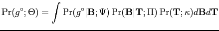
The structural identification of a generic MGRF model in
Eq. (6.2.5) for a given training image
![]() involves the following steps:
involves the following steps:
|
|
|
An MBIM jointly depicts the partial energies of all clique families
in a texture, from which a characteristic pixel neighbourhood
![]() can be estimated.
can be estimated.
A generic MGRF model allows an arbitrary structure of pairwise pixel
interactions, but the longest interaction to recover depends on the
size of each individual training image in practice. Without loss of
generality, Markov property is assumed such that all the neighbours
of a pixel ![]() are limited into a large search window
are limited into a large search window
![]() centred on the pixel. So,
centred on the pixel. So,
![]() . In order to capture the periodicity structure of a
texture, the search window must be large enough to cover at least a
few repetitions. Empirically, the window size is chosen between
. In order to capture the periodicity structure of a
texture, the search window must be large enough to cover at least a
few repetitions. Empirically, the window size is chosen between
![]() and
and ![]() of the size of the training texture. The empirical
rule accounts for the need of enough samples for each clique family
to reliably collect GLCHs and estimate energies.
of the size of the training texture. The empirical
rule accounts for the need of enough samples for each clique family
to reliably collect GLCHs and estimate energies.
Let the width and the height of a search window
![]() be
denoted
be
denoted
![]() and
and
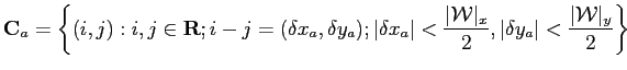
![]() respectively. A
clique family
respectively. A
clique family
![]() in a texture has the maximum
displacement of
in a texture has the maximum
displacement of
![]() and
and
![]() along
along ![]() and
and ![]() axes respectively, so
that,
axes respectively, so
that,
Formally, an MBIM is a 2D function,
![]() , which maps a search window
, which maps a search window
![]() onto
real-valued partial energies
onto
real-valued partial energies
![]() . A two-step procedure is
involved in computing the partial energy for each clique family.
First, a GLCH matrix is collected for the family, by convolving the
displacement vector with the image. Second, the partial energy is
computed by Eq. (6.3.4) from the collected
statistics. A generic MGRF model only counts on the relative
frequency,
. A two-step procedure is
involved in computing the partial energy for each clique family.
First, a GLCH matrix is collected for the family, by convolving the
displacement vector with the image. Second, the partial energy is
computed by Eq. (6.3.4) from the collected
statistics. A generic MGRF model only counts on the relative
frequency,
![]() , of
co-occurrence of every two grey levels
, of
co-occurrence of every two grey levels ![]() and
and ![]() ,
,
![]() , so the resulting matrix has a dimensionality of
, so the resulting matrix has a dimensionality of
![]() . To have statistically meaningful
estimates for small training images (e.g.,
. To have statistically meaningful
estimates for small training images (e.g.,
![]() ) and also due to computational restrictions, a texture is
typically converted into a 16-level gray-scale image before further
processing [38].
) and also due to computational restrictions, a texture is
typically converted into a 16-level gray-scale image before further
processing [38].
Since the relative energy is sufficient for ranking clique families,
the first approximation of relative partial energy
![]() in
Eq. (6.3.4) is used to approximate the
`real' partial energy
in
Eq. (6.3.4) is used to approximate the
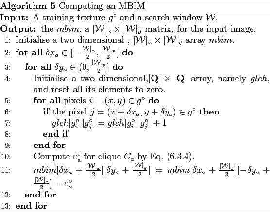
`real' partial energy ![]() in forming an MBIM. The procedure of
computing the MBIM is outlined by Algorithm 5.
in forming an MBIM. The procedure of
computing the MBIM is outlined by Algorithm 5.
An MBIM is symmetric about the origin ![]() , because a clique
family
, because a clique
family
![]() has the same pixel
interaction as the clique family
has the same pixel
interaction as the clique family
![]() . It also should be noted
that there is no such a clique family with a zero displacement
vector
. It also should be noted
that there is no such a clique family with a zero displacement
vector ![]() .
.
The major computation in constructing an MBIM comes from convolution
operation in collecting the GLCH statistics for each clique family
of the image. The process involves quadratic time complexity of
![]() , which depends on the sizes of
both the searching window and the training image.
, which depends on the sizes of
both the searching window and the training image.
An MBIM can be represented graphically either by a 2D bitmap or on a
3D surface, in which each coordinate
![]() represents a clique family
represents a clique family
![]() ,
and the corresponding scalar value represents the partial energy
,
and the corresponding scalar value represents the partial energy
![]() of that family. Figure 6.2 shows a few
examples of 2D representation of MBIMs by grey-level images, with
the partial energy encoded by intensity, i.e. dark intensities
correspond to higher-energy clique families, light intensities
correspond to lower-energy clique families. In
Figs 6.3 and 6.4, the
MBIMs are rendered on a 3D surface, where the
of that family. Figure 6.2 shows a few
examples of 2D representation of MBIMs by grey-level images, with
the partial energy encoded by intensity, i.e. dark intensities
correspond to higher-energy clique families, light intensities
correspond to lower-energy clique families. In
Figs 6.3 and 6.4, the
MBIMs are rendered on a 3D surface, where the ![]() values represent
real-valued partial energies.
values represent
real-valued partial energies.
An MBIM reveals several important properties of the clique families in a texture, which helps to recover a characteristic neighbourhood and identify texels from a texture. Experimental comparisons have shown that the more accurate potential estimates in Appendix A produce quite similar MBIMs to those with the potentials of Eq. (6.3.3). For simplicity, below, only the latter estimates are used.
![\includegraphics[scale=0.9]{mbim-grid.eps}](img380.png)
|
The characteristic neighbourhood for a generic MGRF model consists of a group of the most energetic clique families and represents most probably pixel interactions in a texture.
The simplest approach to estimating the structure is to select most energetic clique families by using a threshold of partial energy [37,36]. But the selection of threshold is largely heuristic and the statistical interplay between clique families have not been taken into account.
An alternative sequential approach in [107] selects each
next characteristic clique family by comparing the training GLCHs to
those for an image sampled from the MGRF with the currently
estimated neighbourhood. Since each step involves image sampling
(generation) and re-collection of the GLCHs, the process is very
computationally complex, i.e. to find a neighbourhood structure
![]() , the time complexity is
, the time complexity is
![]() where
where ![]() is the
expected number of steps, which, at least, theoretically
is the
expected number of steps, which, at least, theoretically ![]() grows
exponentially with
grows
exponentially with
![]() although it is limited
to a few hundred steps empirically to generate a single MGRF sample
using the MCMC process of pixel-wise stochastic relaxation.
although it is limited
to a few hundred steps empirically to generate a single MGRF sample
using the MCMC process of pixel-wise stochastic relaxation.
The structural identification simplifies selection of the characteristic neighbourhood due to the observation that most energetic clique families form isolated clusters (or blobs) in the MBIMs shown in Figs 6.3 and 6.4. From the statistical point of view, the clique family having maximum energy in each cluster is related to locally the most probable pixel interaction. Pixel interactions represented by other clique families in the vicinity are also likely but with lower probability. This indicates variations of neighbourhood structure at different locations of an image. The size and shape of the clusters reflect the degree of local variations and could be used to measure texture homogeneity, i.e. a strict homogeneous texture should have a smaller cluster.
It is reasonable to use the local maximum of each cluster as a representative clique family for a local region. A two-step approach is proposed to find these local maxima. First, all the significant clusters are identified from the MBIM, and second, the clique family having the maximal partial energy in each cluster is added into the characteristic neighbourhood.
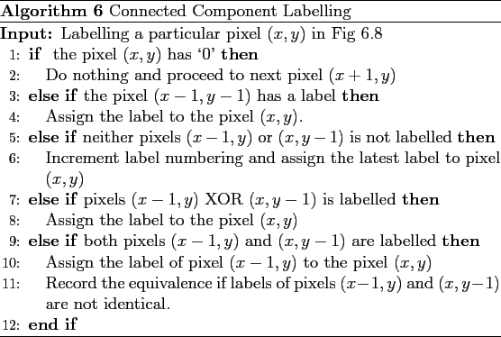
Most MBIMs have their corresponding histograms of partial energies as a unimodal distribution, i.e. each histogram is positively skewed and has a single peak at the lower energy end, as in Fig 6.6. This allows to apply a unimodal thresholding algorithm [87] to determine a threshold that separates high-energy clique families from the majority of low-energy ones. Consequently, clusters formed by high-energy families are isolated and can be easily identified by grouping connected clique families using the classic connected-component labelling algorithm [86]. A local maximum is then identified by as the clique family with maximal energy from each cluster.
![\framebox{
\includegraphics[scale=0.5]{unimodal.eps}
}](img388.png) |
The thresholding algorithm draws a straight line from the peak of the histogram to the last non-empty bin. The threshold is at the point on the histogram curve having the maximal distance to the straight line. The algorithm is illustrated in Fig 6.7.
For simplicity, the structural identification assumes a uniform geometric structure for all texels in a texture, i.e. the same pixel interactions are applicable at every location in the image. The geometric structure is statistically the most probable one, i.e. the central tendency if consider a distribution of all possible texel's structures. This simplification is implied by the assumption of translational-invariant pixel interaction in a generic MGRF model.
The geometric structure of texels in a texture is derived from the characteristic neighbourhood consisting of local maxima of clusters. Structures for regular and stochastic textures are specified in separate ways, due to the different nature of two texture classes.
Figures 6.3 and 6.4 schematically illustrate several texels for stochastic and regular textures, respectively, where each texture has a distinguishing geometric structure of texels corresponding to the spatial distribution of clusters in the MBIM.
The geometric structure can be used as a mask for sampling (retrieving) texels from a texture. For example, one can superimpose a mask at an arbitrary location on an image, the group of signals covered by the mask are related to a particular texel for the texture. In a same way, texels of the same structure but different signals are retrieved at different locations from the image. Since in our experiments most texels look like a bunch of image signals, this sampling method is also called in [40] bunch sampling.
![\includegraphics[scale=0.3]{d34_tess.eps}](img393.png)
|
Repetitions of various texels create periodicity, structure and symmetry in a texture. A special placement rule is derived to model spatial relationship between texels, i.e. how the image locations of multiple occurrences of a single texel or different texels are related in forming a texture pattern.
In a stochastic texture, texels appear with no explicit placement rules and have mostly weak spatial interrelations. As shown later, a synthetic texture of this class can be formed by sampling, repeating and randomly placing of the distinct training texels.
In contrast, a regular texture involves strict placement rules reflecting the underlying strong periodicity. Due to the assumption of translation-invariant pixel interaction, only translation symmetry is taken into account in estimating the placement rule for texels for textures in this class.
In a regular texture, there exists a underlying placement grid
guiding the repetitions of texels. Each grid cell is a compact
bounding parallelogram around a texel mask, specified by parameters
![]() , where
, where ![]() and
and ![]() are guiding angles that give orientations of cell sides with respect
to the image coordinate axes, and
are guiding angles that give orientations of cell sides with respect
to the image coordinate axes, and ![]() and
and ![]() are the side lengths,
i.e. the mask's spans along the orientational directions. The
bounding parallelogram could be decided using an invariant fitting
algorithm, which is related to a canonical frame of the texel
mask [103]. Figure 6.9 shows a hexagonal
texel mask of texture D34, its bounding parallelogram and related
parameters
are the side lengths,
i.e. the mask's spans along the orientational directions. The
bounding parallelogram could be decided using an invariant fitting
algorithm, which is related to a canonical frame of the texel
mask [103]. Figure 6.9 shows a hexagonal
texel mask of texture D34, its bounding parallelogram and related
parameters ![]() . In general, the grid with parallelogram cells
represents any five possible types of translation lattice known in
the theory of wallpaper groups for repeated
patterns [89].
. In general, the grid with parallelogram cells
represents any five possible types of translation lattice known in
the theory of wallpaper groups for repeated
patterns [89].
The placement grid is related to a coordinate system with non-orthogonal basis vectors, which leads to a hexagonal tessellation of the image plane [94]. Figure 6.10 shows a tessellation of texture D34 in line with a placement grid defined by the cell in Fig 6.9.
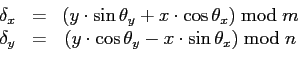
Figure 6.10 also shows that, with the
tessellation, each texel is associated with a relative shift,
![]() , of its centre
, of its centre ![]() , with respect to
the origin made coincident with the centre of the closest grid cell:
, with respect to
the origin made coincident with the centre of the closest grid cell:
The placement rule is to repeat each training texel at arbitrary locations having the same relative shift with respect to the placement grid. Due to an infinite number of absolute image locations related to a same relative shift, the rule reflects translation symmetry of regular textures. It also suggests that an arbitrarily large texture can be synthesised by expanding the image lattice in line with the infinite placement grid.
The structural identification yields a texel-based description that characterises a texture by texels and placement rules of their arrangement. Recently, several similar works describing a texture by its primitive elements have been proposed. However, instead of `texel', the majority of the known works use an alternative term `texton', suggested by Julesz, to refer to small objects or characteristic regions that comprise a texture. Research shows that only the difference in textons or in their density can be detected pre-attentively by human early visual system [54].
Motivated by Julesz's texton theory, a few recent works [63,71,100,101,102] employ a filter-based spectral analysis technique to relate textons to the centres of clusters in filter responses of a stack of training images. Conceptually, each texton, as a feature descriptor in the spectral domain, represents a particular statistical spectral feature describing repetitive patterns of a texture in the spatial domain. All the textons form a global texton dictionary, or a feature space, allowing to characterise a texture by an empirical probability distribution of the textons, i.e. the frequency with which each texton in the dictionary occurs in the texture. A nearest-neighbour classifier with similarity metrics based on chi-square distance between texton distributions, can classify textures into different categories. But since only the occurrences of a texton are taken into account, spatial information about relationships between the textons is completely lost in the description.
A texton-based generative model of image in [112] contains
local constructs at three levels: pixels, image bases, and textons.
An image base is a group of pixels forming a micro geometric element
like a circle or a line. In this case, a texton is actually a
mini-template consisting of a number of image bases of some
geometric and photometric configurations. In an image, these textons
are meaningful objects like stars or birds that could be observed.
The probability model with parameters
![]() is specified as follows:
is specified as follows:
The MLE of the model parameters ![]() or the estimates
minimising the Kullback-Leibler divergence are learned using a
data-driven MCMC algorithm. Due to the complex likelihood function,
the experiments were limited in several aspects in order to keep the
problem tractable: (i) only a small number of image bases in
the global base map, e.g., a few Laplacian-of-Gaussian and Gabor
base functions; (ii) the spatially independent textons for
simplicity, and (iii) only very simple textures with a
priori obvious image bases and textons.
or the estimates
minimising the Kullback-Leibler divergence are learned using a
data-driven MCMC algorithm. Due to the complex likelihood function,
the experiments were limited in several aspects in order to keep the
problem tractable: (i) only a small number of image bases in
the global base map, e.g., a few Laplacian-of-Gaussian and Gabor
base functions; (ii) the spatially independent textons for
simplicity, and (iii) only very simple textures with a
priori obvious image bases and textons.
In both above mentioned and most of other known texton-based approaches, spatial relationship among the textons is either neglected or otherwise too difficult to represent. In contrast, the proposed structure identification provides a much simpler but yet more complete texture description.
![\includegraphics[width=2.2in]{texel-simple.eps}](img319.png)
![\includegraphics[scale=0.7]{d4.bmp.eps}](img320.png)
![\includegraphics[scale=0.7]{d4.m.bmp.eps}](img321.png)
![\includegraphics[scale=0.7]{d6.bmp.eps}](img322.png)
![\includegraphics[scale=0.7]{d6.m.bmp.eps}](img323.png)
![\includegraphics[scale=0.7]{d12.bmp.eps}](img324.png)
![\includegraphics[scale=0.7]{d12.m.bmp.eps}](img325.png)
![\includegraphics[scale=0.7]{d20.bmp.eps}](img326.png)
![\includegraphics[scale=0.7]{d20.m.bmp.eps}](img327.png)
![\includegraphics[scale=0.7]{d24.bmp.eps}](img328.png)
![\includegraphics[scale=0.7]{d24.m.bmp.eps}](img329.png)
![\includegraphics[scale=0.7]{d52.bmp.eps}](img330.png)
![\includegraphics[scale=0.7]{d52.m.bmp.eps}](img331.png)
![\includegraphics[scale=0.7]{d66.bmp.eps}](img332.png)
![\includegraphics[scale=0.7]{d66.m.bmp.eps}](img333.png)
![\includegraphics[scale=0.7]{d76.bmp.eps}](img334.png)
![\includegraphics[scale=0.7]{d76.m.bmp.eps}](img335.png)
![\includegraphics[scale=0.7]{d105.bmp.eps}](img336.png)
![\includegraphics[scale=0.7]{d105.m.bmp.eps}](img337.png)
![\includegraphics[scale=0.7]{d77.bmp.eps}](img338.png)
![\includegraphics[scale=0.7]{d77.m.bmp.eps}](img339.png)
![\includegraphics[scale=0.7]{d29.bmp.eps}](img344.png)
![\includegraphics[scale=0.7]{bark0009.bmp.eps}](img345.png)
![\includegraphics[scale=0.35]{d29MBIM.eps}](img346.png)
![\includegraphics[scale=0.35]{bark09MBIM.eps}](img347.png)
![\framebox{
\includegraphics[scale=0.42]{d29texel.eps}
}](img342.png)
![\framebox{
\includegraphics[scale=0.42]{bark09texel.eps}}](img343.png)
![\includegraphics[scale=0.7]{d34.bmp.eps}](img350.png)
![\includegraphics[scale=0.7]{d101.bmp.eps}](img351.png)
![\includegraphics[scale=0.35]{d34MBIM.eps}](img352.png)
![\includegraphics[scale=0.35]{d101MBIM.eps}](img353.png)
![\framebox{
\includegraphics[scale=0.42]{d34texel.eps}
}](img348.png)
![\framebox{
\includegraphics[scale=0.42]{d101texel.eps}}](img349.png)
![\framebox{
\includegraphics[scale = 0.35]{d29_hist.eps}
}](img384.png)
![\framebox{
\includegraphics[scale = 0.35]{bark09_hist.eps}}](img385.png)
![\framebox{
\includegraphics[scale = 0.35]{d34_hist.eps}
}](img386.png)
![\framebox{
\includegraphics[scale = 0.35]{d101_hist.eps}}](img387.png)
![\includegraphics[scale=0.6]{connectedcomp.eps}](img389.png)
![\includegraphics[scale=0.4]{d34_grid.eps}](img392.png)