Model Identification

Identification of a generic MGRF model in Eq. (6.2.5) involves recovering a characteristic neighbourhood $\mathcal{N}$ and estimating the potential vector $\mathbf{V}^\mathsf{T}$, from image signal statistics $\mathbf{F}{({g})}$ given by an image ${g}$.

There is a chicken-and-egg problem in the identification; On the one hand, the potentials $\mathbf{V}^\mathsf{T}$ need to be known to compute the partial energy in Eq. (6.2.3) for selecting clique families into the characteristic neighbourhood. But, on the other hand, the potentials $\mathbf{V}^\mathsf{T}$ require an explicit interaction structure $\mathcal{N}$ before can be computed. An analytic first approximation of potentials is proposed to work around the problem. The idea is to first compute an approximation of potentials for recovering the characteristic neighbourhood, and then to refine the potentials using a more accurate method (e.g., stochastic approximation) based on the estimated neighbourhood. Model identification of a generic MGRF model has three main steps,

1. Compute the analytic first approximation of potentials
2. Recover the characteristic neighbourhood $\mathcal{N}$.
3. Potential refinement via stochastic approximation.

Analytic First Approximation of Potentials

Model parameters $\mathbf{V}^\mathsf{T}$ in Eq. (6.2.5) are estimated by computing MLE  $\mathbf{V}^*$. Given a neighbourhood $\mathcal{N}$ and a training image ${g}^{\circ}$, the log-likelihood function $\ell(\mathbf{V}\vert{g}^{\circ})=\log P({g}^{\circ}\vert\mathbf{V})$ of the potential is:

$$\ell(\mathbf{V}\vert{g}^{\circ})=\mathbf{V}^\mathsf{T}\mathbf{F}(... ...\sum_{{g}\in\mathcal{S}} \exp\left( \mathbf{V}^\mathsf{T}\mathbf{F}({g})\right)$$ (6.3.1)

The MLE  $\mathbf{V}^*$ can not be obtained analytically because the second item in Eq. (6.3.1) involves the entire configuration space.

In a generic MGRF model, a quadratic approximation to the log-likelihood function $\ell(\mathbf{V}\vert{g}^{\circ})$ based on Taylor series is applied to simplify the log likelihood function and allows to analytically compute an first approximation of potentials, $\mathbf{V}^{\circ} \approx \mathbf{V}$. For a clique family $\mathbf{C}_a$, the first approximation of potential $\mathbf{V}_a^{\circ}$ is given by,

$$\begin{array}{lll} \mathbf{V}_a^{\circ}&=&\{V_a^{\circ}(q,s),... ...dot \left(F_a(q,s \mid {g}^{\circ})-M{(q,s)}\right) \end{array}$$ (6.3.2)

where ${g}^{\circ}$ is the training image, $M(q,s)=\frac{1}{{Q}^2}$ is the centred marginal probabilities of signal co-occurrences for the IRF, and $\rho_{a}=\frac{\vert\mathbf{C}_a\vert}{\vert\mathbf{R}\vert}$ gives the relative size of the clique family $\mathbf{C}_a$ with respect to the lattice size. The scaling factor $\lambda_{0}$ is calculated using the same GLCHs and centred grey level histogram (GLH). A more detailed derivation of the first approximation of potentials can be found in [37,36,38]. More accurate model identifications are given in Appendix A.

The first approximation of potentials might not be adequate for computing an accurate posterior distribution $Pr({g}^{\circ})$, but it gives a sub-optimal estimate of partial energy for each clique family and allows to identify the characteristic neighbourhood of the model.

Characteristic Neighbourhood

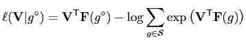
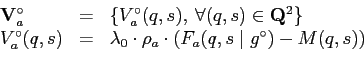
The characteristic neighbourhood represents an interaction structure constituted by the most energetic clique families. Most of clique families in a texture have rather low partial energy, and therefore related pixel interactions have little or no impact on texture patterns. In contrast, only a small number of most energetic clique families are major contributors to a texture. This observation suggests only the most energetic clique families should be included in the interaction structure.

The selection of clique families is based on partial energy which measures the probabilistic strength of related pixel interaction. Given the first approximation of potential $\mathbf{V}_a^{\circ}(q,s)$ in Eq. (6.3.2) and the partial energy $E_{a}$ in Eq. (6.1.3), an approximation of partial energy for a clique family $\mathbf{C}_a$ can be computed from a training sample ${g}^{\circ}$ by:

$$E_{a}^{\circ}({g}\vert V_{a})=\vert\mathbf{C}_a\vert \cdot \lambd... ...mathbf{Q}^2}(F_a(q,s \mid {g}^{\circ})-M{(q,s)})\cdot F_a(q,s \mid {g}^{\circ})$$ (6.3.3)

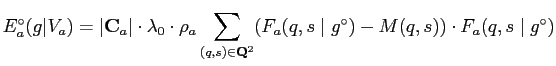
Since the dimension of the image lattice $\vert\mathbf{R}\vert$ and the factor $\lambda_{0}$ are constant, the approximation of partial energy can be simplified further to a relative partial energy, $\mathsf{\varepsilon}_{a}^{\circ}({g}\vert V_{a})$, for simplicity.

$$\mathsf{\varepsilon}_{a}^{\circ}({g}\vert V_{a})={\vert\mathbf{C}... ...athbf{Q}^2} (F_a(q,s \mid {g}^{\circ})-M{(q,s)})\cdot F_a(q,s \mid {g}^{\circ})$$ (6.3.4)

The relative partial energy $\mathsf{\varepsilon}_{a}^{\circ}({g}\vert V_{a})$ provides a relative measure of contribution and allows to rank all the clique families accordingly. The most characteristic clique families can be found by using a threshold in the simplest case. To a good approximation, the relative partial energies of all clique families are assumed to follow a Gaussian distribution. Therefore, the threshold $\theta$ is heuristically decided by a function of the mean $\bar{\mathsf{\varepsilon}}$ and the standard deviation $\sigma_{\mathsf{\varepsilon}}$ of the Gaussian [37].

$$\theta=\bar{\mathsf{\varepsilon}}+c\sigma_{\mathsf{\varepsilon}}$$ (6.3.5)

However, this over-simplified method of determining the interaction structure by using a threshold does not take statistical interplay among clique families into account, which might result in neglecting some important clique families. In other words, only statistical independent clique families should be included into the interaction structure [39]. In another approach, clique families are selected iteratively based on their statistical impact to the probability distribution [107]. In this method, the interaction structure grows from a single clique family with maximum energy and only one clique family is selected at each iteration. The statistical impact of a clique family is defined by the change to the probability distribution after adding the family into the structure. This method involves computational expensive operations of re-sampling distribution and re-collecting GLCH statistics at each step, but the recovered structure is more adequate and considerably smaller than the structure obtained by thresholding.

Potential Refinement

Given the obtained interaction structure, the first approximation of potentials should be refined in order to determine the posterior probability distribution $Pr({g})$ in Eq. (6.2.5).

A stochastic approximation [85] algorithm is applied to iteratively refine the potential toward the MLE $\mathbf{V}^*$. Basically, the process constructs a Markov chain and updates the potential at each iteration $t$ based on the following equation [38],

$$\mathbf{V}^{[t]}=\mathbf{V}^{[t-1]}+\lambda^{[t]}{(\mathbf{F}({g}^{[0]})-\mathbf{F}({g}^{[t]}))}$$ (6.3.6)

$$\mathbf{V}^{[0]}=\mathbf{V}_a^{\circ}$$ (6.3.7)

Here, ${g}^{[t]}$ is an image generated at step $t$ by sampling the previous probability distribution, $Pr^{[t-1]}({g} \mid \mathbf{V}^{[t-1]})$, using Gibbs sampling [34] or Metropolis algorithm [77]. $\lambda^{[t]}=\lambda^{[0]}\frac{c_0+1}{c_1+c_2{t}}$ is the scale factor. The initial scale $\lambda^{[0]}$ and the control parameters $c_0$, $c_1$ and $c_2$ can be decided either analytically or empirically.

The termination condition of the process is given as follows,

$$\vert\mathbf{V}^{[t]}-\mathbf{V}^*\vert < \epsilon$$ (6.3.8)

where $\epsilon$ is a predefined threshold.

The stochastic approximation is rather computational-intensive, which usually takes more than a few hundred steps to attain convergence. Speed of convergence and the comparison with an alternative MCMC based technique, called Controllable Simulated Annealing(CSA), are discussed in [38],