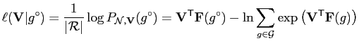
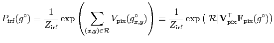
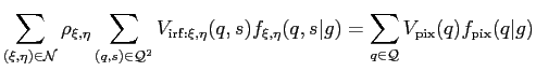
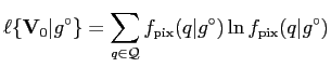
Recall Eq. (6.2.5). Given the neighbourhood
![]() , the specific log-likelihood of the potential:
, the specific log-likelihood of the potential:
Starting from a potential
![]() producing an IRF, the
maximum likelihood estimate (MLE) of the potential is approximated
by generalising the analytical approach proposed in [38].
producing an IRF, the
maximum likelihood estimate (MLE) of the potential is approximated
by generalising the analytical approach proposed in [38].

The approximate solution in [38] presumes the simplest IRF
(denoted below
![]() ) with zero potential
) with zero potential
![]() . It results in equal marginal
probabilities
. It results in equal marginal
probabilities
![]() of independent signals
of independent signals
![]() ;
;
![]() , over
, over
![]() and
equiprobable
images in Eq. (6.2.5):
and
equiprobable
images in Eq. (6.2.5):
![]() .
In this case
.
In this case
![]() and all pairwise
co-occurrence probabilities are equal:
and all pairwise
co-occurrence probabilities are equal:
![]() .
.
Let
![]() be the vector of the scaled marginal
co-occurrence probabilities for the
be the vector of the scaled marginal
co-occurrence probabilities for the
![]() :
:
![]() where
where
![]() is the
is the ![]() -vector of
unit components. Let
-vector of
unit components. Let
![]() be the
vector of the centred scaled empirical co-occurrence probabilities
be the
vector of the centred scaled empirical co-occurrence probabilities
![]() for the image
for the image ![]() , i.e.
, i.e.
![]() ,
,
where
![]() for all
for all
![]() .
.
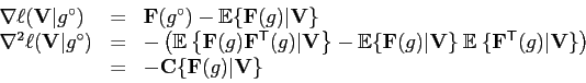
Then the log-likelihood gradient is
![]() and the covariance matrix
and the covariance matrix
![]() is closely approximated
by the scaled diagonal covariance matrix
is closely approximated
by the scaled diagonal covariance matrix
![]() for the independent co-occurrence distributions:
for the independent co-occurrence distributions:
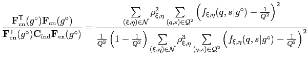
![]() where
where
![$ \mathbf{C}_\mathrm{ind} = \frac{1}{Q^2}\left(1 -
\frac{1}{Q^2}\right)\mathsf{Diag} \left[ \rho_{\xi,\eta} \mathbf{u}:
(\xi,\eta)\in\mathcal{N} \right] $](img587.png) .
.
 .
.
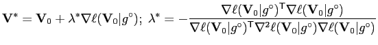
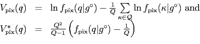
Assuming the centred potential,
![]() , it is easily shown
that the actual potential MLE and its first approximation obtained
for a training image
, it is easily shown
that the actual potential MLE and its first approximation obtained
for a training image ![]() much as in
Proposition A.0.2 but for the IRF in Eq. (A.0.5)
are, respectively,
much as in
Proposition A.0.2 but for the IRF in Eq. (A.0.5)
are, respectively,
Table A.1 presents both the estimates in a special case
when one intensity,
![]() , has the empirical probability
, has the empirical probability
![]() and all remaining
intensities are equiprobable,
and all remaining
intensities are equiprobable,
![]() ;
;
![]() . The
estimates are given in function of
. The
estimates are given in function of ![]() and the relative
probability
and the relative
probability
![]() . For small
. For small ![]() , both the
estimates are close to each other except for
, both the
estimates are close to each other except for
![]() . But
for larger
. But
for larger ![]() , the approximate MLE of Eq. (A.0.4)
exceeds considerably the actual one so that the approximation may be
intolerably inaccurate for the MGRFs, too.
, the approximate MLE of Eq. (A.0.4)
exceeds considerably the actual one so that the approximation may be
intolerably inaccurate for the MGRFs, too.
| Relative probabilities |
|||||||||||||||
|
|
1.0 | 2.0 | 5.0 | 10 | 20 | 50 | 100 | 200 | 500 | |
|
|
|
||
| 2 | e | 0.00 | 0.67 | 1.33 | 1.64 | 1.81 | 1.92 | 1.96 | 1.98 | 1.99 | 2.00 | 2.00 | 2.00 | 2.00 | |
| a | 0.00 | 0.35 | 0.80 | 1.15 | 1.50 | 1.96 | 2.30 | 2.65 | 3.11 | 3.45 | 4.61 | 5.76 | |||
| |
0.50 | 0.67 | 0.83 | 0.91 | 0.95 | 0.98 | 0.99 | 1.00 | 1.00 | 1.00 | 1.00 | 1.00 | 1.00 | ||
| e | 0.00 | 0.80 | 2.00 | 2.77 | 3.30 | 3.70 | 3.84 | 3.92 | 3.97 | 3.98 | 4.00 | 4.00 | 4.00 | ||
| a | 0.00 | 0.52 | 1.21 | 1.73 | 2.25 | 2.93 | 3.45 | 3.97 | 4.66 | 5.18 | 6.91 | 8.63 | |||
| |
0.25 | 0.40 | 0.63 | 0.77 | 0.87 | 0.94 | 0.97 | 0.98 | 0.99 | 1.00 | 1.00 | 1.00 | 1.00 | ||
| e | 0.00 | 0.89 | 2.67 | 4.24 | 5.63 | 6.88 | 7.40 | 7.69 | 7.87 | 7.94 | 7.99 | 8.00 | 8.00 | ||
| a | 0.00 | 0.61 | 1.41 | 2.01 | 2.62 | 3.42 | 4.03 | 4.64 | 5.44 | 6.04 | 8.06 | 10.1 | |||
| |
0.13 | 0.22 | 0.42 | 0.59 | 0.74 | 0.88 | 0.93 | 0.97 | 0.99 | 0.99 | 1.00 | 1.00 | 1.00 | ||
| e | 0.00 | 0.94 | 3.20 | 5.76 | 8.69 | 12.1 | 13.8 | 14.8 | 15.5 | 15.8 | 16.0 | 16.0 | 16.0 | ||
| a | 0.00 | 0.65 | 1.51 | 2.16 | 2.81 | 3.67 | 4.32 | 4.97 | 5.83 | 6.48 | 8.63 | 10.8 | |||
| |
0.06 | 0.12 | 0.25 | 0.40 | 0.57 | 0.77 | 0.87 | 0.93 | 0.97 | 0.99 | 1.00 | 1.00 | 1.00 | ||
| e | 0.00 | 0.97 | 3.56 | 7.02 | 11.9 | 19.4 | 24.2 | 27.6 | 30.1 | 31.0 | 31.9 | 32.0 | 32.0 | ||
| a | 0.00 | 0.67 | 1.56 | 2.23 | 2.90 | 3.79 | 4.46 | 5.13 | 6.02 | 6.69 | 8.92 | 11.2 | |||
| |
0.03 | 0.06 | 0.14 | 0.24 | 0.39 | 0.62 | 0.76 | 0.87 | 0.94 | 0.97 | 1.00 | 1.00 | 1.00 | ||
| e | 0.00 | 0.98 | 3.76 | 7.89 | 14.7 | 27.8 | 38.9 | 48.4 | 56.7 | 60.2 | 63.6 | 64.0 | 64.0 | ||
| a | 0.00 | 0.68 | 1.58 | 2.27 | 2.95 | 3.85 | 4.53 | 5.22 | 6.12 | 6.80 | 9.07 | 11.3 | |||
| |
0.02 | 0.03 | 0.07 | 0.14 | 0.24 | 0.44 | 0.61 | 0.76 | 0.89 | 0.94 | 0.99 | 1.00 | 1.00 | ||
| e | 0.00 | 0.99 | 3.88 | 8.41 | 16.5 | 35.4 | 55.8 | 77.9 | 102. | 113. | 126. | 128. | 128. | ||
| a | 0.00 | 0.69 | 1.60 | 2.28 | 2.97 | 3.88 | 4.57 | 5.26 | 6.17 | 6.85 | 9.14 | 11.4 | |||
| |
0.01 | 0.02 | 0.04 | 0.07 | 0.14 | 0.28 | 0.44 | 0.61 | 0.80 | 0.89 | 0.99 | 1.00 | 1.00 | ||
| e | 0.00 | 1.00 | 3.94 | 8.69 | 17.7 | 41.1 | 71.4 | 112. | 169. | 204. | 250. | 255. | 256. | ||
| a | 0.00 | 0.69 | 1.60 | 2.29 | 2.98 | 3.90 | 4.59 | 5.28 | 6.19 | 6.88 | 9.17 | 11.5 | |||
| |
0.00 | 0.01 | 0.02 | 0.04 | 0.07 | 0.16 | 0.28 | 0.44 | 0.66 | 0.80 | 0.98 | 1.00 | 1.00 | ||
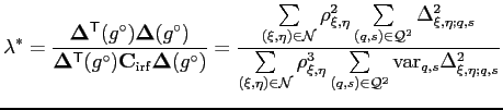
Let
![]() denote the
difference between the empirical and actual signal co-occurrence
probabilities for the IRF identified from the image
denote the
difference between the empirical and actual signal co-occurrence
probabilities for the IRF identified from the image ![]() . Let
. Let
![]() be the variance of the latter probability:
be the variance of the latter probability:
![]() . Then
the gradient
. Then
the gradient
![]() of the log-likelihood is the
of the log-likelihood is the
![]() -vector of the scaled differences:
-vector of the scaled differences:
![]() and the covariance matrix
and the covariance matrix
![]() is closely approximated
by the scaled diagonal matrix
is closely approximated
by the scaled diagonal matrix
![]() where
where
![]() is the
is the ![]() -vector of
the variances:
-vector of
the variances:
![]() .
.
 |
(A.0.7) |