A wide range of MGRF models have been proposed [6,45,20,34,13,7,75,37,113] over the last several decades. Essentially, an MGRF model considers an image as a realisation of a Markov random field (MRF). A major advantage of MGRF models is that they allow to derive a global texture description by specifying local properties of textures. In this section, fundamental theories of MRFs, Gibbs distribution, and MGRF-based texture modelling are presented.
Consider a two dimensional ![]() lattice
lattice
![]() . If each site
. If each site
![]() is associated with
a random variable
is associated with
a random variable
![]() , one obtains a
random field,
, one obtains a
random field,
![]() [34]. A digital image
[34]. A digital image
![]() could be considered as a realisation or a random
sample of the random field
could be considered as a realisation or a random
sample of the random field
![]() , i.e. a particular
assignment of a set of signal values to all sites of the lattice
, i.e. a particular
assignment of a set of signal values to all sites of the lattice
![]() [41].
[41].
Since the random variables in a random field are considered
statistically dependent, a joint probability distribution of random
variables for an image ![]() defines a probability model of
the image from the statistical viewpoint. The joint distribution is
denoted by
defines a probability model of
the image from the statistical viewpoint. The joint distribution is
denoted by ![]() or simply
or simply ![]() , representing the chance
to observe the image given the configuration
space
, representing the chance
to observe the image given the configuration
space
![]() of all images associated with the random field.
of all images associated with the random field.
A desired joint probability distribution for an image model should
yields mostly or almost zero probability for all the images except a
subset-of-interest around a given training image. Formally, the
distribution function is expected to be similar to ![]() -function
having its maximum mode on or in a close vicinity of the training
image.
-function
having its maximum mode on or in a close vicinity of the training
image.
If no prior knowledge is available, a probability model must
enumerate all possible labelling of the lattice in order to derive a
joint distribution. This is an intractable task, because the
configuration space
![]() has combinatorial cardinality,
has combinatorial cardinality,
![]() . If each site is assumed to be
independent of any others, i.e. an independent random
field (IRF), a probability model is specified by the joint
probability distribution,
. If each site is assumed to be
independent of any others, i.e. an independent random
field (IRF), a probability model is specified by the joint
probability distribution,
![]() .
The probability is uninformative and the resulting image
model is not particular useful.
.
The probability is uninformative and the resulting image
model is not particular useful.
Most real-life probability models assume certain local dependency
among random variables/image pixels. A conditional
probability of a pixel ![]() given all other pixels
given all other pixels ![]() ,
denoted by
,
denoted by
![]() , is commonly exploited to
represent local dependency. In this case, a random field is
represented by a undirected graph
, is commonly exploited to
represent local dependency. In this case, a random field is
represented by a undirected graph
![]() in which each graph
vertex represents a random variable while an edge represents
statistical dependency between two connected vertices. The absence
of an edge between two vertices in the graph implies that the
associated random variables are conditionally independent given all
other random variables.
in which each graph
vertex represents a random variable while an edge represents
statistical dependency between two connected vertices. The absence
of an edge between two vertices in the graph implies that the
associated random variables are conditionally independent given all
other random variables.
Within such a graphical structure, a probability model for a random
field could be factorised into a normalised product of strictly
positive, real-valued potential functions defined on subsets
of connected random variables in
![]() . Each subset
form a local neighbourhood system with a spatial
configuration, and the image corresponds to a global
configuration of all random variables. A potential function has no
probabilistic meaning other than representing constraints on the
local configuration on which it is defined [60]. This
graphical representation indicates that the probability distribution
of an image can be specified in terms of potential functions of
local neighbourhood, which reduces the complexity of a global image
modelling problem. This is the main idea of applying MRF models for
texture modelling.
. Each subset
form a local neighbourhood system with a spatial
configuration, and the image corresponds to a global
configuration of all random variables. A potential function has no
probabilistic meaning other than representing constraints on the
local configuration on which it is defined [60]. This
graphical representation indicates that the probability distribution
of an image can be specified in terms of potential functions of
local neighbourhood, which reduces the complexity of a global image
modelling problem. This is the main idea of applying MRF models for
texture modelling.
MGRF-based texture models have been successfully applied into texture analysis [6,45,20,34,13,7,75,37,113], texture classification and segmentation [23,24,73], and texture synthesis [29,104,65,59]. In this section, definitions and general theories related to an MGRF are introduced.
Here, the first condition is known as the positivity of an MRF,
which is trivial. The second condition is known as Markov
property or Markovianity. The equivalence, between the
conditional probability
![]() of the signal value
of the signal value
![]() given all the other signal values
given all the other signal values
![]() and the conditional probability
and the conditional probability
![]() of signal value
of signal value ![]() given all signal values of the
neighbouring sites
given all signal values of the
neighbouring sites
![]() , suggests that the pixel value at
a site in the image is only dependent of that of its neighbouring
sites.
, suggests that the pixel value at
a site in the image is only dependent of that of its neighbouring
sites.
The Markov property describes conditional dependence of image signals within a local neighbourhood system, which is proved to be useful in capturing and modelling usually highly localised and coherent texture features. Another appealing property of an MRF is that, by the Hammersley-Clifford theorem [42], an MRF can be characterised by a global Gibbs distribution.
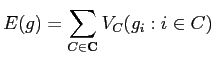
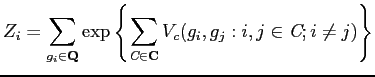
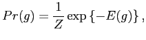
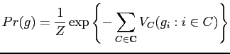
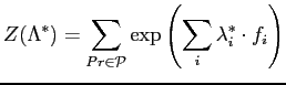
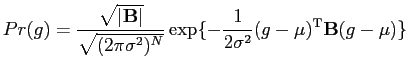
In general, a Gibbs distribution takes the following form,
The partition function is also known as the normalising constant. Because it is defined over the entire configuration space, the partition function is intractable. This would arise difficulties in parameter estimation of the density function of a Gibbs distribution. A random field having a Gibbs distribution is called a Gibbs random field (GRF).
A Gibbs distribution is usually defined with respect to
cliques, i.e. proper subgraphs of a neighbourhood graph on
the lattice. A clique is a particular spatial configuration of
pixels, in which all its members are statistically dependent of each
other. All the statistical links between pixels in an image
constitute a neighbourhood graph or system denoted by
![]() .
Cliques and the neighbourhood system model spatial geometry of pixel
interactions, which are particularly useful in texture modelling.
All spatial configurations of cliques related to the 8-nearest
neighbourhood system are shown in Fig 5.2. Formally, a
clique is defined as follows,
.
Cliques and the neighbourhood system model spatial geometry of pixel
interactions, which are particularly useful in texture modelling.
All spatial configurations of cliques related to the 8-nearest
neighbourhood system are shown in Fig 5.2. Formally, a
clique is defined as follows,
The number of pixels in a clique specifies the statistical order of
a Gibbs distribution and the related texture model . For texture
modelling, first-order and second-order cliques are frequently used,
because higher-order cliques causes too much computational
complexity. First-order and second-order cliques over the image
lattice
![]() are denoted as by
are denoted as by
![]() and
and
![]() , respectively:
, respectively:
Statistical dependence between pixels within a clique is also
referred to pixel interaction. Let a non-constant function
![]() denote the strength of the pixel
interaction in a clique
denote the strength of the pixel
interaction in a clique ![]() . The function
. The function ![]() is also known
as clique potential. The energy function
is also known
as clique potential. The energy function ![]() in
Eq. (5.2.2) could be factorised into the sum of clique
potentials
in
Eq. (5.2.2) could be factorised into the sum of clique
potentials
![]() over the set
over the set ![]() , so that
, so that
Hammersley-Clifford Theorem asserts that a random field is a Markov random field if and only if the corresponding joint probability distribution is a Gibbs distribution [42]. The theorem, also known as MRF-Gibbs distribution equivalence, has been proved by Grimmett [41], Besag [6], and Gemans [34] respectively.
The theorem establishes the equivalence between an MRF and a GRF,
which provides a factorisation of a global probability distribution
![]() in terms of local interaction functions with respect to
cliques. Particularly, the joint probability
in terms of local interaction functions with respect to
cliques. Particularly, the joint probability ![]() and the
conditional probability
and the
conditional probability
![]() can specify each
other.
can specify each
other.
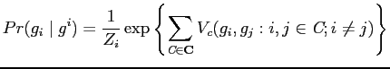
By the Hammersley-Clifford Theorem, the conditional probability of
an MRF
![]() can be specified in following
form [34], in terms of clique potential,
can be specified in following
form [34], in terms of clique potential, ![]() .
.
 |
(5.2.6) |
Similarly, the clique potential ![]() of the Gibbs distribution can
also be derived from the conditional probability
of the Gibbs distribution can
also be derived from the conditional probability
![]() of an MRF but in a more complicated form. An MRF is uniquely
related to a normalised potential, called the canonical
potential [64].
of an MRF but in a more complicated form. An MRF is uniquely
related to a normalised potential, called the canonical
potential [64].
In summary, Markov-Gibbs equivalence provides a theoretical basis for texture modelling based on MGRFs, which allows to employ the global characteristics in modelling while the local characteristics in processing a field [34].
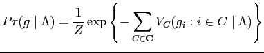
The parametric form of the Gibbs distribution in
Eq. (5.2.2) with parameters ![]() is given as
follows:
is given as
follows:
Model identification is usually formulated as a global optimisation problem that maximises either the entropy or the likelihood of probability distributions.
If domain knowledge and observed statistics are represented as a set of constraints, Maximum entropy (MaxEnt) principle could be applied in estimating parameters of model distributions.
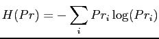
The MaxEnt principle states that a desired prolixity distribution should be assigned by maximising the entropy while subject to a set of constraints [52,60]. The entropy of a probability distribution measures uncertainty [92], which is denoted by:
The MaxEnt principle is formulated as an optimisation problem that
maximises ![]() ,
,
This constrained optimisation problem can be solved by maximising following Lagrangian,
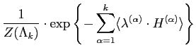
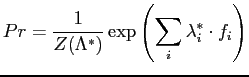
The resulting MaxEnt distribution is as follows,
Similar forms of the probability distributions in Eqs. (5.2.7) and (5.2.11) suggest that the Gibbs distribution of an MGRF belongs to the exponential families and is an MaxEnt distribution. Actually, all distributions belonging to so-called exponential families [2] possess the MaxEnt property. In particular, a generic MGRF model is specified by an MaxEnt distribution constrained by the training sufficient statistics, i.e. co-occurrence frequency distributions.
The MaxEnt principle suggests an alternative approach to texture modelling. One can first select sufficient statistics to characterise textures and then infer the MaxEnt distribution subject to the constraints that the marginal probability of sufficient statistics with respect to the model should match the empirical probability of the same statistics in the training data. As introduced later, both the generic MGRF [37,36] and FRAME [113] models use this strategy to derive their MaxEnt distributions. But the former derivation refers to the exponential families, while the latter approach does not mention the exponential families at all and derives their sufficient features from the scratch.
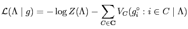
Maximum likelihood estimation (MLE) is one of the most commonly used procedure for estimating unknown parameters of a distribution. MLE is based on likelihood principle which suggests model parameters should maximising the probability of occurrence of the observation, e.g., a training image, given the configuration space.
Given the parametric form of a Gibbs distribution
![]() in Eq. (5.2.7), the likelihood function for
in Eq. (5.2.7), the likelihood function for
![]() is given by,
is given by,
If
![]() is differentiable, the parameters
is differentiable, the parameters
![]() for the MLE, given a training image
for the MLE, given a training image
![]() ,
is computed by solving
,
is computed by solving
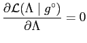
However, due to the intractable normalisation constant
![]() in Eq. (5.2.13), numerical techniques such as
Markov Chain Monte Carlo (MCMC) algorithms have to be used for
estimating
in Eq. (5.2.13), numerical techniques such as
Markov Chain Monte Carlo (MCMC) algorithms have to be used for
estimating
![]() . As shown in [4], the MaxEnt
method is equivalent to the MLE in estimating distributions in
exponential families and therefore Gibbs distributions.
. As shown in [4], the MaxEnt
method is equivalent to the MLE in estimating distributions in
exponential families and therefore Gibbs distributions.
An MCMC algorithm allows to simulate a probability distribution by
constructing a Markov chain with the desired distribution as its
stationary distribution. A Markov chain, defined over a set of
sequential states, is an one-dimensional case of an MRF. Each state
of the chain relates to a particular assignment of all involves
random variables on which the stationary distribution is defined.
The transition from a state ![]() to
to ![]() is controlled by the
transition probability,
is controlled by the
transition probability,
![]() , indicating
Markov property of the chain,
, indicating
Markov property of the chain,
The MCMC algorithm iteratively updates the Markov chain based on the transition probability from a state to another state. Eventually, the chain attains the state of equilibrium when the joint probability distribution for the current state approaches the stationary distribution. The parameters that leads to the stationary distribution are considered as the model parameters learnt for the particular training image.
In the case of texture modelling, each state of an Markov chain relates to an image as a random sample drawn from the joint distribution. The image obtained at the state of equilibrium is expected to resemble the training image. In other words, parameter estimation via MCMC algorithms simulates the generative process of a texture and therefore synthesises textures.
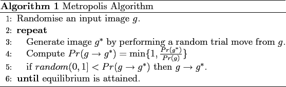
Each state of a Markov chain is obtained by sampling a probability distribution. Among various sampling techniques, Metropolis algorithm [77] and Gibbs sampler [34] are two most well-known ones. Metropolis algorithm provides a mechanism to explore the entire configuration space by random walk. At each step, the algorithm performs a random modification to the current state to obtain a new state. The new state is either accepted or rejected with a probability computed based on energy change in the transition. The states generated by the algorithm form a Markov chain. Algorithm 1 outlines a basic Metropolis algorithm.
Gibbs sampler is a special case of the Metropolis algorithm, which
generates new states by using univariate conditional
probabilities [64]. Because direct sampling from the complex
joint distribution of all random variables is difficult, Gibbs
sampler instead simulate random variables one by one from the
univariate conditional distribution. A univariate conditional
distribution involves only one random variable conditioned on the
rest variables having fixed values, which is usually in a simple
mathematical form. For instance, the conditional probability
![]() for an MRF is a univariate conditional
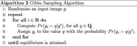
distribution. A typical Gibbs sampling algorithm [34] is
outlined in Algorithm 2.
for an MRF is a univariate conditional
distribution. A typical Gibbs sampling algorithm [34] is
outlined in Algorithm 2.
In summary, an MCMC method learns a probability distribution
![]() by simulating the distribution via a Markov chain. The
Markov chain is specified by three probabilities, an initial
probability
by simulating the distribution via a Markov chain. The
Markov chain is specified by three probabilities, an initial
probability
![]() , the transition probability
, the transition probability
![]() , and the stationary probability
, and the stationary probability
![]() . The MCMC process is specified by the following equation,
. The MCMC process is specified by the following equation,
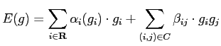
Auto-models [6] are the simplest MGRF models in texture analysis, which are defined over rather simple neighbourhood systems with ``contextual constraints on two labels'' [64]. The Gibbs energy function for an auto-model only involves first- and second-order cliques, having the following general form [25],
There are several variations of auto-models, such as auto-binomial model [20] and auto-normal model [13,18], each of which assumes slightly different models of pair-wise pixel interaction.
Hence, the conditional distribution is given by,
| (5.2.17) |
By Markov-Gibbs equivalence, the Gibbs distribution is specified by the energy function,
 |
(5.2.18) |
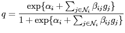
In an auto-binomial model, model parameters are the sets
![]() and
and
![]() . The set
. The set
![]() has a
fixed size, but the size of the set
has a
fixed size, but the size of the set
![]() is related to
the order of the selected neighbourhood system. To simplify
parameter estimation, one could reduce the number of parameters, for
instance, by assuming a uniform value
is related to
the order of the selected neighbourhood system. To simplify
parameter estimation, one could reduce the number of parameters, for
instance, by assuming a uniform value ![]() for all the sites
and using only the simplest neighbourhood system, i.e 4- or
8-nearest neighbours.
for all the sites
and using only the simplest neighbourhood system, i.e 4- or
8-nearest neighbours.
![$\displaystyle Pr({g}_i \mid {g}^i)=\frac{1}{\sqrt{2\pi{\sigma}^2}}\exp\{-\frac{1}{2{\sigma}^2}[{g}_i-\mu({g}_i \mid {g}^i)]^2\}$](img152.png) |
(5.2.19) |
Here,
![]() is the conditional mean
and
is the conditional mean
and ![]() is the conditional variance (standard deviation).
is the conditional variance (standard deviation).
By Markov-Gibbs equivalence, an auto-normal model is specified by the following joint probability density:
An auto-normal model defines a continuous Gaussian MRF. The model
parameters,
![]() ,
,
![]() , and
, and ![]() , can be
estimated using either MLE or pseudo-MLE methods [7]. In
addition, a technique representing the model in the spatial
frequency domain [13] has also been proposed for
parameter estimation.
, can be
estimated using either MLE or pseudo-MLE methods [7]. In
addition, a technique representing the model in the spatial
frequency domain [13] has also been proposed for
parameter estimation.
FRAME (short for Filters, Random Fields, and Maximum Entropy) [113] is an MGRF model constructed from the empirical marginal distributions of filter responses based on the MaxEnt principle. The FRAME model is derived based on Theorem. 5.2.1, which asserts that the joint probability distribution of an image is decomposable into the empirical marginal distributions of related filter responses. The proof of the theorem is given in [113].
The theorem suggests that the joint probability distribution
![]() could be inferred by constructing a probability
could be inferred by constructing a probability
![]() whose marginal distributions
whose marginal distributions
![]() match
with the same distributions of
match
with the same distributions of ![]() . Although, theoretically,
an infinite number of empirical distributions (filters) are involved
in the decomposition of a joint distribution, the FRAME model
assumes that only a relative small number of important filters (a
filter bank),
. Although, theoretically,
an infinite number of empirical distributions (filters) are involved
in the decomposition of a joint distribution, the FRAME model
assumes that only a relative small number of important filters (a
filter bank),
![]() , are
sufficient to the model distribution
, are
sufficient to the model distribution ![]() . Within an MaxEnt
framework, by Eq. (5.2.8), the modelling is formulated as
the following optimisation problem,
. Within an MaxEnt
framework, by Eq. (5.2.8), the modelling is formulated as
the following optimisation problem,
 |
(5.2.21) |
subject to constraints:
In Eq. (5.2.22),
![]() denotes the
marginal distribution of
denotes the
marginal distribution of ![]() with respect to the filter
with respect to the filter
![]() at location
at location ![]() , and by definition,
, and by definition,
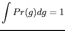
The second constraint in Eq. (5.2.23) is the
normalising condition of the joint probability distribution
![]() .
.
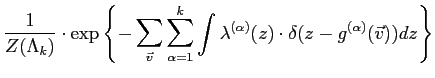
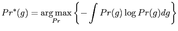
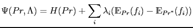
The MaxEnt distribution ![]() are found by maximising the
entropy using Lagrange multipliers,
are found by maximising the
entropy using Lagrange multipliers,
 |
|||
![$\displaystyle + \sum_{\alpha =1}^{k}
\lambda^{(\alpha)} \cdot\left(
{\mathcal{E}}_{Pr}[\delta(z-{g}^{(\alpha)}(v))]-Pr^{(\alpha)}(z)\right)$](img181.png) |
|||
 |
 |
 |
||
 |
 |
|||
 |
|||
 |
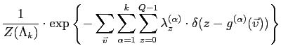
The discrete form of
![]() is derived by the
following transformations,
is derived by the
following transformations,
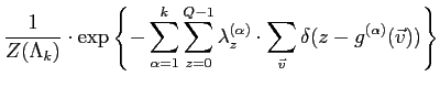
Here, the vector of piecewise functions,
![]() and
and
![]() ,
represent the histogram of filtered image
,
represent the histogram of filtered image
![]() and the
Lagrange parameters, respectively.
and the
Lagrange parameters, respectively.
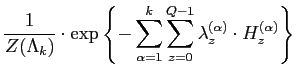
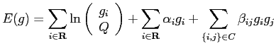
As shown in Eq. (5.2.25), the FRAME model is specified by a
Gibbs distribution with the marginal empirical distribution
(histogram) of filter responses as its sufficient statistics. The
Lagrange multipliers ![]() are model parameters to estimate
for each particular texture. Typically, the model parameters are
learnt via stochastic approximation which updates parameter
estimates iteratively based on the following equation,
are model parameters to estimate
for each particular texture. Typically, the model parameters are
learnt via stochastic approximation which updates parameter
estimates iteratively based on the following equation,
![\includegraphics[width=4in]{cliques.eps}](img86.png)
![$\displaystyle Pr({g}^{[n]}) = Pr({g}^{[0]})\prod_{t=1}^{n} Pr({g}^{[t]} \mid {g}^{[t-1]})$](img137.png)
![$\displaystyle Pr^{(\alpha)}_{v}(z)=\int\;\int_{{g}^{(\alpha)}(v)=z}{Pr({g})d{g}}={\mathcal{E}}_{Pr}[\delta(z-{g}^{(\alpha)}(v))]$](img172.png)