Texture synthesis has been under intensive study for decades. Most of recent synthesis approaches are based on MGRF models of textures. Assuming that visual similarity follows the proximity of signal statistics [35], these methods replicates observed sufficient statistics from a training into a synthetic image in order to approximate the perceived visual similarity between images.
An MGRF model is generative, because a new texture could be generated by simulating the underlying stochastic process of a texture that the model describes. Such a synthesis process is coincident with the statistical identification of an MGRF model via MCMC algorithms. Since each state of the Markov chain is related to an image randomly sampled from the current joint distribution, in line with the above assumption, the image at the equilibrium state should be visually similar to a sample of the stationary distribution, i.e. the training sampling. This approach to texture synthesis is so-called model-based. Due to the exponential time complexity of the MCMC algorithms, however, model-based synthesis is rather slow for practical applications.
Non-parametric sampling methods were developed recently for fast texture synthesis. These methods are related to non-parametric analysis in statistics which allows to analyse data without knowing an underlying distribution. In texture synthesis, non-parametric sampling methods avoid building an explicit, parametric probability model (e.g., a Gibbs probability density function) for texture description. Instead, they exploit some local methods, e.g., local neighbourhood matching, for reproducing statistics of the training texture. The main advantage of a method based on non-parametric sampling is that it involves less calculation and provides faster synthesis compared with conventional model-based approaches.
Since MGRF model-based texture synthesis has the same procedure as model identification introduced in the previous section and the synthesis based on a generic MGRF model will be given in Chapter 7, this section only focuses on methods based on non-parametric sampling.
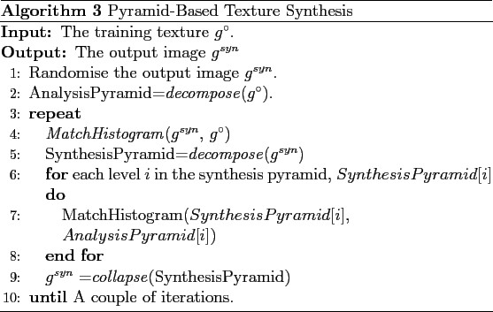
Pyramid-based texture synthesis [Heeger and Bergen] [46] is a very first `fast' algorithm that generates a new texture by matching certain statistics with the training sample. In the method, a texture is decomposed into pyramid-based representations, i.e. an analysis and a synthesis pyramids are constructed from the training and the output textures respectively. The algorithm iteratively refines a synthesised texture by matching its histogram against that of the training texture, and by matching the histogram of each level of the synthesis pyramid with that of the corresponding level of the analysis pyramid. The synthesis process involves mainly image pyramid operations and histogram matching.
There are two basic pyramid operations, namely, reduce and expand. The reduce operation involves filtering and downsampling an image to obtain a new image at the coarser resolution. The expand operation involves upsampling and interpolating an image to obtain an image at the finer resolution. The process of constructing a pyramid from an image is called decompose, which involves continuous reduce operations. While the process of obtaining an image from a pyramid is called collapse, which involves continuous expand operations. The Gaussian, Laplacian, and steerable pyramids are among the most popular ones used for image processing. Gaussian and Laplacian pyramids involve Gaussian and Laplacian-of-Gaussian base functions respectively [11], while steerable pyramid uses wavelet transforms [46], for decomposing an image.
In the pyramid-based texture synthesis, the Laplacian and the steerable pyramids decompose a texture into multiple bands of spatial frequencies and orientations respectively. Each pyramid level represents certain texture features at a particular frequency or orientation. The histogram of each pyramid level is chosen as a descriptor of the related features. The synthesis is based on the idea that a new texture could be generated by matching all the available features (histograms) with the training texture.
where ![]() is the input image,
is the input image,
![]() is the image with a
flat histogram, and
is the image with a
flat histogram, and
![]() is the cumulative
distribution function. Let the histogram of an image
is the cumulative
distribution function. Let the histogram of an image ![]() be
denoted by
be
denoted by
![]() as a function of grey level
as a function of grey level
![]() . The cumulative distribution function
. The cumulative distribution function
![]() of
the image
of
the image ![]() is as follows,
is as follows,
![$\displaystyle \mathcal{P}[ {g} ] = \frac{1}{\vert{g}\vert}\int_{0}^{Q}\mathbf{H}_{{g}}(q)dq$](img215.png) |
(5.3.2) |
Given Eq. (5.3.1), the problem of matching
the histogram of an image ![]() with the desired histogram of the
image
with the desired histogram of the
image
![]() is solved as follows [12],
is solved as follows [12],
In Eq. (5.3.3), the histogram matching
involves two concatenated point operations, where
![]() is the inverse function of
is the inverse function of
![]() . Practically the cumulative
distribution function and its inverse function are discrete, which
could be implemented using lookup tables [46].
. Practically the cumulative
distribution function and its inverse function are discrete, which
could be implemented using lookup tables [46].
The synthesis is based on the assumption that ``matching the pointwise statistics of the pyramid representation does matching some of the spatial statistics of the reconstructed image'' [46]. However, as shown in the experimental results, the method produces satisfactory results on stochastic textures with mainly short-range statistical signal dependence but fails on quasi-periodic or regular textures involving large scale features. This indicates that the chosen statistics (the histogram of a pyramid level) are not sufficient for representing especially long-range spatial features. Another main drawback is that the convergence of the iterative synthesis has not been theoretically justified.
Nevertheless, the pyramid-based method is a very first effort on applying non-parametric technique for texture synthesis. The novelty of this method is in the idea of synthesising texture by matching image signal statistics.
Multi-resolution sampling [22], proposed by DeBonet, also constructs an analysis and a synthesis Guassian/Laplacian pyramids in texture synthesis. But it has two major improvements over the previous method [46]; First, multi-resolution sampling extracts a set of more detailed and sophisticated image features by applying a filter bank onto each pyramid level. Second, multi-resolution sampling explicitly takes the joint occurrence of texture features across multiple pyramid levels into account, while the previous method processes each pyramid level separately.
The method synthesises a texture by first generating a synthesis
pyramid on a top-down, level-by-level basis and then collapsing the
pyramid to obtain a synthetic texture. At each level of the
synthesis pyramid, an image is generated pixel by pixel, each pixel
being directly sampled from the corresponding level of the analysis
pyramid. The sampling process, e.g., selection of pixels, is based
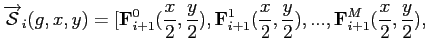
on a similarity measure defined in terms of a parent
structure, associated with each image location ![]() at the level
at the level
![]() of the pyramid for an image
of the pyramid for an image ![]() , as follows [22],
, as follows [22],
A parent structure represents the joint occurrence of
multi-resolution features at a particular image location. The
distance between parent structures provides a similarity measure for
different image locations, i.e. if two locations have similar parent
structures, they are considered indistinguishable [22].
To synthesise a pixel, the algorithm searches the same level of the
analysis pyramid for candidate locations that have the most similar
parent structures to the current one, i.e. the square distance of
each component
![]() between two structures is below a
predefined threshold. Then a randomly selected pixel from the
candidate list is used as the synthesised value.
between two structures is below a
predefined threshold. Then a randomly selected pixel from the
candidate list is used as the synthesised value.
This method introduces a novel constrained sampling technique that generates a new texture using pixels selected from the training image. In fact, a training texture is considered as an exemplar and the synthetic texture as a rearrangement of image signals randomly and coherently sampled from the training one. This technique is also known as non-parametric sampling [29]. Based on the same idea, a variety of methods based on non-parametric sampling techniques have been developed, ranging from pixel-based to the latest patch-based sampling [29,104,65,59,28,78]. Compared to model-based image generation, these techniques provide much faster texture synthesis.
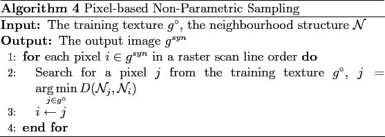
Pixel-based non-parametric sampling [29], proposed by Efros and Leung, constrains pixel sampling using a similarity metric defined with respect to a local neighbourhood system in an MRF.
![\includegraphics[scale=0.65]{pixel-neighbour.eps}](img231.png)
|
The method assumes an MGRF model of textures so that a pixel ![]() only depends on the pixels in a local neighbourhood
only depends on the pixels in a local neighbourhood
![]() . The distance between neighbourhoods
. The distance between neighbourhoods
![]() and
and
![]() , e.g., the
sum-of-square-difference (SSD), provides a metric of pixel
similarity between
, e.g., the
sum-of-square-difference (SSD), provides a metric of pixel
similarity between ![]() and
and ![]() . To synthesise a pixel
. To synthesise a pixel ![]() , the
algorithm searches for a pixel
, the
algorithm searches for a pixel ![]() from the training texture that
minimises the distance between
from the training texture that
minimises the distance between
![]() and
and
![]() ,
and then uses the value of pixel
,
and then uses the value of pixel ![]() for pixel
for pixel ![]() .
.
The constraint to pixel selection is very similar to the multi-resolution sampling approach [22], except that this one is based on a local neighbourhood but the previous one on a hierarchical parent structure. In the multi-resolution sampling, the synthesis has to be carried out in a top-down manner, because a parent structure is defined with respect to higher pyramid levels (see Eq. (5.3.4)). In this method, to maximise the number of synthesised pixels in the neighbourhood of current pixel, the synthesis is performed pixel by pixel in a raster scan-line order. Considering the simplest case that the algorithm synthesises an image from top to bottom and left to right, since only the known parts (already synthesised pixels) of the neighbourhoods are involved in computing the distance, the actual neighbourhood has `L' shape, as shown in Fig 5.3.
The synthesis algorithm is outlined in Algorithm 4,
where
![]() denotes a selected distance
function for neighbourhood comparison.
Figure 5.4 shows synthesised textures by
the pixel-based non-parametric sampling [29].
denotes a selected distance
function for neighbourhood comparison.
Figure 5.4 shows synthesised textures by
the pixel-based non-parametric sampling [29].
In this method, Markov property of a texture is preserved in a non-parametric way; it ranks samples of observed pixel neighbourhoods and selects the closest one based on a similarity metric. Essentially, the sampling attempts to maintain local integrity of texture. This method can have several disadvantages. First, the synthesis grows texture pixel by pixel sequentially, which tends to blur features or to grow small local structures (garbage growing) [29]. Second, the synthesis involves exhaustive search for a pixel having the closest neighbourhood, which could be time consuming especially when a large-size texture or neighbourhood window is involved. Although it outperforms model-based synthesis in synthesis speed, pixel-based non-parametric sampling is still far from real-time. Third, selection of the geometric structure for the local neighbourhood (size and shape) is largely heuristic. Figure 5.5 shows the importance of a correct local neighbourhood (only the size in this example) to the synthesis result of a pixel-based non-parametric sampling method [104]. However, because a local neighbourhood is usually texture-dependent, i.e. related to the characteristics of each individual texture, it might be difficult to find a proper structure without texture modelling,
![\includegraphics[scale=0.32]{pixel-window-size.bmp.eps}](img238.png)
|
A similar pixel-based non-parametric sampling technique, proposed by Wei and Levoy, exploits tree-structured vector quantisation (TSVQ) to speed up neighbourhood searching [104]. This method involves a similarity measure based on a multi-resolution local neighbourhood structure, consisting of pixels from both the current and the next lower levels of an image pyramid. This structure is a mixture of the parent structure in [22] and the local neighbourhood in [29]. By including pixels from an coarser level, it reduces the size of local neighbourhood and thus saves computation time. To avoid the exhaustive neighbourhood searching, this method builds a binary TSVQ tree in which each pixel neighbourhood for the training texture is coded by a node. Since the TSVQ tree is a data structure providing computationally more feasible nearest-point queries, the problem of neighbourhood matching is solved the nearest-point search that traverses the TSVQ tree [104].
Another variation of pixel-based non-parametric sampling, proposed
by Ashikhmin, is for synthesising natural
textures [1]. The method modifies the sampling
process by explicitly accounting for pixel interdependency in the
training image. That is, for a current pixel to be synthesised,
instead of from a random location, the neighbourhood search starts
from the surrounding areas where already-synthesised neighbouring
pixels were sampled in the training image. For example, ``if a pixel
two rows above and one column to the right of current position was
taken from position
![]() in the input sample, the new
candidate is pixel
in the input sample, the new
candidate is pixel
![]() in the input
sample'' [1]. Since it restricts the search space in
a small region, this heuristic greatly reduces the searching time.
In addition, it tends to `follow' coherent local structures (e.g., a
leaf) appeared in many natural textures. The method does not work
well on textures without `any significant amount of high frequency
component' [1]. Since this method tends to follow and
move a group of connected signals (e.g., a small region) from the
training texture onto the synthetic one, the behaviour is similar to
a group of block-based non-parametric sampling techniques.
in the input
sample'' [1]. Since it restricts the search space in
a small region, this heuristic greatly reduces the searching time.
In addition, it tends to `follow' coherent local structures (e.g., a
leaf) appeared in many natural textures. The method does not work
well on textures without `any significant amount of high frequency
component' [1]. Since this method tends to follow and
move a group of connected signals (e.g., a small region) from the
training texture onto the synthetic one, the behaviour is similar to
a group of block-based non-parametric sampling techniques.
Block sampling is a natural extension to the previous pixel-based methods, which improves time efficiency of the synthesis by using image blocks as basic synthesis units. So, instead of pixel by pixel, block sampling synthesises a texture on a block by block basis.
|
However, the method considers a rectangular image patch instead of a single pixel at each step of the synthesis. Each rectangular patch has a boundary zone, being the area surrounding four borders inside the patch (See Fig 5.6 (a)). The difference between boundary zones provides a measure of similarity for two related patches.
Algorithmically, the patched-based sampling is also very similar to the pixel-based algorithm in Algorithm 4. At each step, a patch, which has the closet boundary zone to the patch at the current location, is selected from the training image and is then stitched into the output image such that its boundary zone overlaps with that of the last synthesised patches (See Fig 5.6 (b)). A blending algorithm has to be used in order to smooth the transition between overlapping patches.
This method is generally faster than pixel-based non-parametric sampling, but it has the similar limitations. First, an image patch is usually restricted to be in a rectangular shape, because otherwise a boundary zone is practically difficult to define and to use, i.e. it could be difficult to compare and stitch two irregular boundary zones. Second, the size and the boundary zone of an image patch are two key parameters to the synthesis; the former should be related to the size of local structures for each particular texture, while the latter implies the level of statistical constraints imposed on the sampling process. But, it is still an open challenge to automate the process of finding good parameters for different textures. Third, the method blends overlapping areas, which could blur resulting textures and cause visual artifacts.
|
Formally an optimal cut is found by using dynamic programming or
Dijkstra's algorithm which minimises the minimum cumulative
matching error ![]() along the path [28],
along the path [28],
where ![]() is the cumulative error until the pixel
is the cumulative error until the pixel ![]() along the path, and
along the path, and ![]() is the matching error at pixel
is the matching error at pixel ![]() which is given by the Euclidean distance of signal values at the
pixel between two overlapping patches.
which is given by the Euclidean distance of signal values at the
pixel between two overlapping patches.
In image quilting, since the overlapping area between two rectangular patches is always along one of four sides, the optimal cut only goes either vertically or horizontally through the overlapping area. This limitation might prevent the algorithm from finding a global optimal cut.
The synthesis procedure is similar to a best-first search problem, which selects and cuts the patch that has currently the best evaluation according to a heuristic function. Since the approach doesn't necessarily yield the best global solution, an iterative scheme should also be considered to refine the result towards a optimal global function.
Finding an optimal cut has been formulated by a well established
technique of graph cut in graph theory. Image
quilting [28] exploits one-dimensional graph cut,
i.e. each cut only goes one direction, while this method involves a
two-dimensional case, i.e. each cut goes arbitrarily on a 2D plane.
The graph cut algorithm have a worst-case computational complexity
of ![]() and an average of
and an average of
![]() for a graph with
for a graph with ![]() nodes [59].
nodes [59].
Three methods for selecting patches are investigated in [59]. The simplest and the fastest method is random placement, which places the entire input image into the output image lattice with a random shift each time. The second method, entire patch matching, finds the best transition of the input image by minimising a normalised SSD of the overlapping area between an input and an output images. The third method, sub-patch matching, searches an input image for the best match that minimises a certain distance function between two patches, which is similar to both the patch-based method [65] and image quilting [28].
Image quilting [28] and graph cut[59] first select a patch and then decide which portion of a patch should be merged into the output texture accord to an optimal cut. A technique, namely, cut-primed smart copy reverses the order, which cuts the training image into tiles first followed by tessellating tiles in generating a new texture [78].
Considering an image as a graph with each pixel being a vertex, a cut is a path running through between vertices on the graph. Each cut creates a seam consisting of all the pairs of corresponding vertices separated by the cut either vertically or horizontally, as illustrated in Fig 5.9. An optimal cut should create the lest visible seam. The visibility of a seam is measured by the sum of difference of intensity between each vertex pair along the cut. So, finding an optimal cut is formulated as a shortest path search problem with seam visibility being the cost function. The problem is solved using the classical Dijkstra algorithm [78].
The optimal cuts tessellate an image into small tiles of the same shape. As shown in [78], each tile has both left-to-right and top-to-bottom symmetry, resulted from two different cuts. Therefore, two tiles can be stitched together along one of the four sides resulted from an identical cut. In the synthesis (smart copy) stage, at each step, a tile is selected from the training image and is then stitched into the output image to match existing tiles. Since the cuts minimise the seam visibility between tiles, the resulting texture should also have the minimal seam visibility.
![\includegraphics[scale=0.32]{cut-seam.eps}](img252.png)
|
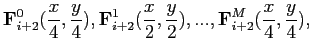
![$\displaystyle \mathbf{F}_{N}^0(\frac{x}{2^N}, \frac{y}{2^N}), \mathbf{F}_{N}^1(...
...c{x}{2^N}, \frac{y}{2^N}),..., \mathbf{F}_{N}^M(\frac{x}{2^N}, \frac{y}{2^N}) ]$](img226.png)
![\includegraphics[scale=0.22]{pixelnonparam.bmp.eps}](img235.png)
![\includegraphics[scale=0.5]{patch-sampling.eps}](img241.png)
![\includegraphics[scale=0.5]{patch-sampling2.EPS}](img242.png)
![\includegraphics[scale=0.7]{quilting.eps}](img243.png)
![\includegraphics[scale=0.7]{quilting1.EPS}](img244.png)
![\includegraphics[scale=0.6]{graph-cut.eps}](img249.png)