FRAME (short for Filters, Random Fields, and Maximum Entropy) [113] is an MGRF model constructed from the empirical marginal distributions of filter responses based on the MaxEnt principle. The FRAME model is derived based on Theorem. 5.2.1, which asserts that the joint probability distribution of an image is decomposable into the empirical marginal distributions of related filter responses. The proof of the theorem is given in [113].
The theorem suggests that the joint probability distribution
![]() could be inferred by constructing a probability
could be inferred by constructing a probability
![]() whose marginal distributions
whose marginal distributions
![]() match
with the same distributions of
match
with the same distributions of ![]() . Although, theoretically,
an infinite number of empirical distributions (filters) are involved
in the decomposition of a joint distribution, the FRAME model
assumes that only a relative small number of important filters (a
filter bank),
. Although, theoretically,
an infinite number of empirical distributions (filters) are involved
in the decomposition of a joint distribution, the FRAME model
assumes that only a relative small number of important filters (a
filter bank),
![]() , are
sufficient to the model distribution
, are
sufficient to the model distribution ![]() . Within an MaxEnt
framework, by Eq. (5.2.8), the modelling is formulated as
the following optimisation problem,
. Within an MaxEnt
framework, by Eq. (5.2.8), the modelling is formulated as
the following optimisation problem,
 |
(5.2.21) |
subject to constraints:
In Eq. (5.2.22),
![]() denotes the
marginal distribution of
denotes the
marginal distribution of ![]() with respect to the filter
with respect to the filter
![]() at location
at location ![]() , and by definition,
, and by definition,
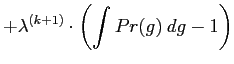
The second constraint in Eq. (5.2.23) is the
normalising condition of the joint probability distribution
![]() .
.
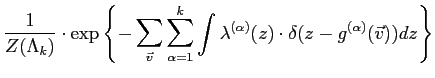
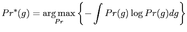
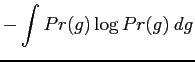
The MaxEnt distribution ![]() are found by maximising the
entropy using Lagrange multipliers,
are found by maximising the
entropy using Lagrange multipliers,
 |
|||
![$\displaystyle + \sum_{\alpha =1}^{k}
\lambda^{(\alpha)} \cdot\left(
{\mathcal{E}}_{Pr}[\delta(z-{g}^{(\alpha)}(v))]-Pr^{(\alpha)}(z)\right)$](img181.png) |
|||
 |
 |
 |
||
 |
 |
|||
 |
|||
 |
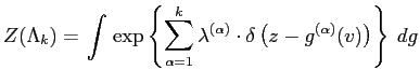
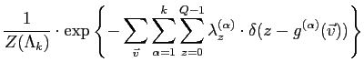
The discrete form of
![]() is derived by the
following transformations,
is derived by the
following transformations,
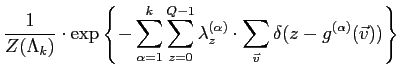
Here, the vector of piecewise functions,
![]() and
and
![]() ,
represent the histogram of filtered image
,
represent the histogram of filtered image
![]() and the
Lagrange parameters, respectively.
and the
Lagrange parameters, respectively.
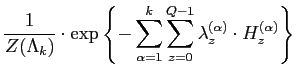
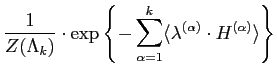
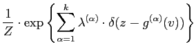
As shown in Eq. (5.2.25), the FRAME model is specified by a
Gibbs distribution with the marginal empirical distribution
(histogram) of filter responses as its sufficient statistics. The
Lagrange multipliers ![]() are model parameters to estimate
for each particular texture. Typically, the model parameters are
learnt via stochastic approximation which updates parameter
estimates iteratively based on the following equation,
are model parameters to estimate
for each particular texture. Typically, the model parameters are
learnt via stochastic approximation which updates parameter
estimates iteratively based on the following equation,
![$\displaystyle Pr^{(\alpha)}_{v}(z)=\int\;\int_{{g}^{(\alpha)}(v)=z}{Pr({g})d{g}}={\mathcal{E}}_{Pr}[\delta(z-{g}^{(\alpha)}(v))]$](img172.png)