Auto-normal Models

[13,18] assume that the conditional probability $Pr({g}_i \vert {g}^i)$ of a pixel is a normal distribution over an $N \times N$ neighbourhood, which is specified as follows,

$$Pr({g}_i \mid {g}^i)=\frac{1}{\sqrt{2\pi{\sigma}^2}}\exp\{-\frac{1}{2{\sigma}^2}[{g}_i-\mu({g}_i \mid {g}^i)]^2\}$$ (5.2.19)

Here, 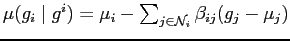$\mu({g}_i \mid {g}^i)=\mu_i-\sum_{j \in \mathcal{N}_i}\beta_{ij}({g}_j-\mu_j)$ is the conditional mean and $\sigma$ is the conditional variance (standard deviation).

By Markov-Gibbs equivalence, an auto-normal model is specified by the following joint probability density:

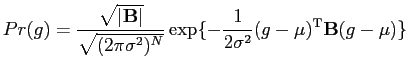$$Pr({g})=\frac{\sqrt{\vert\mathbf{B}\vert}}{\sqrt{(2\pi{\sigma}^2)... ...c{1}{2{\sigma}^2}({g}-\mathbf{\mu})^{\mathrm{T}}\mathbf{B}({g}-\mathbf{\mu}) \}$$ (5.2.20)

where $\mathbf{\mu}$ is an $N \times 1$ vector of the conditional means, and $\mathbf{B}$ is an $N \times N$ interaction matrix with unit diagonal elements, the off diagonal element at the position $(i,j)$ being $-\beta_{ij}$. Since the model distribution in Eq. (5.2.20) is Gibbsian and also Gaussian, an auto-normal model is also known as a Gaussian-Markov random field model.

An auto-normal model defines a continuous Gaussian MRF. The model parameters, $\mathbf{B}$, $\mathbf{\mu}$, and $\sigma$, can be estimated using either MLE or pseudo-MLE methods [7]. In addition, a technique representing the model in the spatial frequency domain [13] has also been proposed for parameter estimation.