Bunch Sampling

The bunch sampling algorithm is based on the results of the structural identification of a generic MGRF model, i.e, the geometric structure and the placement rule derived from a training texture. The geometric structure is used as a mask for sampling texels from the training image, while the placement rule guides the placement of each texel into the synthetic texture. The bunch sampling is similar to the methods based on non-parametric sampling in also transferring and rearranging image signals sampled from the training image into the synthetic one.

For a regular texture, the locations of a texel in the training and the synthetic images are related in order to preserve the placement rule. That is, the two locations have a same relative shift with respect to the estimated placement gird tessellating both images. But for a stochastic texture without an explicit placement rule, each texel is copied to a random location in the synthetic image.

Such a retrieve-and-place procedure repeats until the entire image plane of a new texture is fully covered. Since each step is independent of any previous steps, the synthesis is non-causal.

Algorithm Details

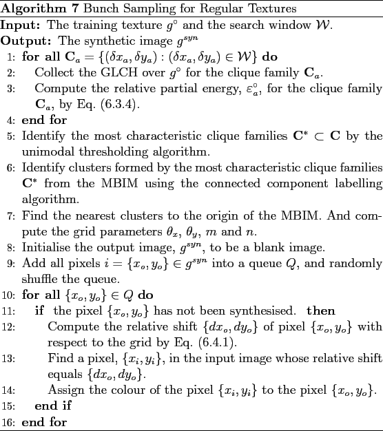
The bunch sampling algorithm for synthesising a regular texture is outlined in Algorithm 7. Generally, the algorithm might be divided into an analysis stage (from lines 0 to 0) and a synthesis stage (from lines 0 to 0).

Analysis Stage

involves collecting the GLCH statistics from a training image and computing partial energy for each clique family to form an MBIM( lines 0 to 0), followed by analysing the resulting MBIM to derive the geometric structure and the placement grid for texels, specified by four grid parameters ( lines 0 to 0).

Synthesis Stage

involves selecting a sampling location of training texels for each synthesis location in line with the placement grid (line 0) and transferring a selected texel onto the output image (line 0). The process of sampling and transferring loops until the entire image plane of the synthetic texture is fully covered (lines. 0 to 0).

Implementation Issues

A few issues regarding implementing the algorithm are discussed below.

Signal Collisions.

In synthesis of a stochastic texture, signal collision might happen when a texel has to be placed into a region that has been partly synthesised. A simple heuristic rule of preserving the already synthesised signals is applied to resolve signal collisions [40].

Texel Selection.

Since most of textures are not strictly homogeneous, a stack of different texels might be associated with a same relative shift reflecting local variations of textures. Two strategies could be used for texel selection in the synthesis. The first method is to compute an approximate Bayesian estimate of texels, based on the maximum marginal posterior (MMP) probabilities of image signals by superposing all associated texels, for each relative shift. The resulting estimate represents the most probable texel at each relative position and is used in texture synthesis. The second method is to select a random texel from the stack as a representative for each relative shift. Synthesis results with both methods are shown and discussed in the next section.

Synthesis of a Colour Texture.

To date most of texture analysis methods have been limited only to grey level images. For instance, a generic MGRF model is usually restricted to 16 grey levels because otherwise model creation and identification become computationally too expensive. A possible approach is to process each channel as a grey-image separately and then to combine the retrieved information [107]. But integrating different colour channels might require computational intensive iterative optimisation procedure. The bunch sampling assumes that texture features are invariant to the colour distribution in an image, so that it converts a colour texture to a grey level image for analysis, i.e. the geometric structure and placement rules of texels are estimated from only the intensity channel of the image. But, at the synthesis stage, the original colour texture is used as a source of texels for sampling. In so doing, colour texels are retrieved and used as construction units to generate a new colour texture. In this case, the synthesis of a colour texture has no much difference from the synthesis of a grey-level one except an extra step needed for converting the training textures from RGB space into grey levels. Since the approach neglects all information preserved in colour channels (hue and saturation), it might fail on certain textures in which texture features are relevant to the distribution of colours. Nevertheless, for most of colour textures used in our experiments, this simple method produces generally good results.

Time Complexity.

The bunch sampling is a fast synthesis algorithm compared to other major synthesis techniques. At the analysis stage, the running time for computing the grid parameters includes the time for both collecting the GLCHs and performing a spatial analysis of the MBIM. Similar to a un-partitioned convolution algorithm, collecting the GLCHs for all clique families inside $\mathcal{W}$ over a training image ${g}^{\circ}$ involves quadratic time complexity, proportional to $\vert{g}^{\circ}\vert\cdot\vert\mathcal{W}\vert$. Since typically a search window has a size proportional to the training image, e.g., $\vert\mathcal{W}\vert = \vert{g}^{\circ}\vert/3$, the time complexity is roughly $O({\vert{g}^{\circ}\vert}^2)$. The running time for the spatial analysis of an MBIM is $O(\vert\mathcal{W}\vert)$, which is linear to the window size. Therefore, the overall time complexity of the analysis stage is $O({\vert{g}^{\circ}\vert}^2)$.

At the synthesis stage, the running time for synthesising each pixel is constant, if a hash table is built to store signal values for each relative shift at a pre-processing stage so that the synthesis of a pixel involves only an operation of querying the hash table. So the time complexity for synthesising the entire texture is $O(\vert{g}^{syn}\vert)$. Building the hash table requires to scan the training image ${g}^{\circ}$ pixel by pixel in a raster scanline order, which has time complexity of $O(\vert{g}^{\circ}\vert)$. Usually $\vert{g}^{\circ}\vert<\vert{g}^{syn}\vert$. Therefore, the overall time complexity at the synthesis stage is still $O(\vert{g}^{syn}\vert)$, which is linearly proportional to the size of the synthetic image.

Figure 7.2: Synthesis of regular textures by bunch sampling: The sizes of training textures, MBIMs, and synthetic textures are $128\times 128$, $125\times 125$ and $360\times360$, respectively. The training textures are taken from [82,8].

MBIM
	D6

MBIM
	D14

MBIM
	D20

MBIM
	D34

MBIM
	D52

MBIM
	D101

MBIM
	D102

MBIM
	Tile07

Figure 7.3: Synthesis of stochastic textures by bunch sampling: The sizes of training textures, MBIMs, and synthetic textures are $128\times 128$, $125\times 125$ and $360\times360$, respectively. The training textures are taken from [82,8].

MBIM
	D4

MBIM
	D24

MBIM
	Bark0009

MBIM
	Water0002

MBIM
	Flower0004

MBIM
	Metal0005

MBIM
	Grass01

MBIM
	Fabric0016

Figure 7.4: Synthesis of colour textures by bunch sampling: The sizes of training textures, MBIMs, and synthetic textures are $128\times 128$, $125\times 125$ and $360\times360$, respectively. The training textures are taken from  [65].

MBIM
	Cans

MBIM
	Weave

MBIM
	Dots

MBIM
	Floor

MBIM
	Flowers

MBIM
	Flora

MBIM
	Knit

MBIM
	Design