Parameter Estimation via MCMC

An MCMC algorithm allows to simulate a probability distribution by constructing a Markov chain with the desired distribution as its stationary distribution. A Markov chain, defined over a set of sequential states, is an one-dimensional case of an MRF. Each state of the chain relates to a particular assignment of all involves random variables on which the stationary distribution is defined. The transition from a state $t$ to $t+1$ is controlled by the transition probability, $Pr({g}^{[t]} \mid {g}^{[t-1]})$, indicating Markov property of the chain,

$$Pr({g}^{[t]} \mid {g}^{[u]}, u \neq t)=Pr({g}^{[t]} \mid {g}^{[t-1]})$$ (5.2.14)

The MCMC algorithm iteratively updates the Markov chain based on the transition probability from a state to another state. Eventually, the chain attains the state of equilibrium when the joint probability distribution for the current state approaches the stationary distribution. The parameters that leads to the stationary distribution are considered as the model parameters learnt for the particular training image.

In the case of texture modelling, each state of an Markov chain relates to an image as a random sample drawn from the joint distribution. The image obtained at the state of equilibrium is expected to resemble the training image. In other words, parameter estimation via MCMC algorithms simulates the generative process of a texture and therefore synthesises textures.

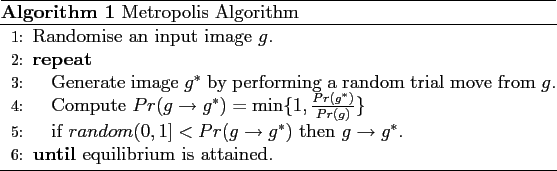
Each state of a Markov chain is obtained by sampling a probability distribution. Among various sampling techniques, Metropolis algorithm [77] and Gibbs sampler [34] are two most well-known ones. Metropolis algorithm provides a mechanism to explore the entire configuration space by random walk. At each step, the algorithm performs a random modification to the current state to obtain a new state. The new state is either accepted or rejected with a probability computed based on energy change in the transition. The states generated by the algorithm form a Markov chain. Algorithm 1 outlines a basic Metropolis algorithm.

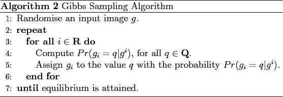
Gibbs sampler is a special case of the Metropolis algorithm, which generates new states by using univariate conditional probabilities [64]. Because direct sampling from the complex joint distribution of all random variables is difficult, Gibbs sampler instead simulate random variables one by one from the univariate conditional distribution. A univariate conditional distribution involves only one random variable conditioned on the rest variables having fixed values, which is usually in a simple mathematical form. For instance, the conditional probability $Pr({g}_i\vert{{g}^i})$ for an MRF is a univariate conditional distribution. A typical Gibbs sampling algorithm [34] is outlined in Algorithm 2.

In summary, an MCMC method learns a probability distribution $Pr({g})$ by simulating the distribution via a Markov chain. The Markov chain is specified by three probabilities, an initial probability $Pr({g}^{[0]})$, the transition probability $Pr({g}^{[t]} \mid {g}^{[t-1]})$, and the stationary probability $Pr({g})$. The MCMC process is specified by the following equation,

$$Pr({g}^{[n]}) = Pr({g}^{[0]})\prod_{t=1}^{n} Pr({g}^{[t]} \mid {g}^{[t-1]})$$ (5.2.15)