Visible colours as linear combinations of the primary RGB components
Colour is one of the most widely used visual features in multimedia context and image / video retrieval, in particular. To support communication over the Internet, the data should compress well and be suitable for heterogeneous environment with a variety of the user platforms and viewing devices, large scatter of the user's machine power, and changing viewing conditions. The CBIR systems are not aware usually of the difference in original, encoded, and perceived colours, e.g., differences between the colorimetric and device colour data (Shi & Sun, 2000).
Colour is a subjective human sensation of visible light depending on an intensity and a set of wavelengths associated with the electromagnetic spectrum. The composition of wavelengths specifies chrominance of visible light for human visual system. The chrominance has two attributes: hue and saturation. The hue is characterised by the dominant wavelength(s) in the composition, and the saturation measures the purity of a colour. A pure colour has 100% of saturation, whereas all shades of colourless (grey) light, e.g. white light, have 0% of saturation.
The sensed colour varies considerably with 3D surface orientation, camera viewpoint, and illumination of the scene, e.g., positions and spectra of illuminating sources. Also, human colour perception is quite subjective as regarding perceptual similarity. To design formal colour descriptors, one should specify a colour space, its partitioning, and how to measure similarity between colours. An absolute colour space (see Wikipedia definition) defines unambiguous colours that are independent of external factors, but most of the popular colour spaces below (e.g. RGB or HSI) are not absolute, although they can be made absolute by more precise definitions of or standards for their elements (e.g. sRGB). Absolute color spaces like a L*a*b* defines an exact abstract colour that can be precisely reproduced when an accurate device is viewed in the right condition.
Colour is a subjective visual characteristic describing how perceived electromagnetic radiation F(l) is distributed in the range of wavelengths l of visible light [380 nm ... 780 nm]. A colour space is a multidimensional space of colour components. Human colour perception combines the three primary colours: red (R) with the wavelength l=700 nm, green (G) with the wavelength l=546.1 nm, and blue (B) with the wavelength l=435.8 nm. Any visible wavelength L is sensed as a colour obtained by a linear combination of the three primary colours (R, G, B) with the particular weights cR( l ), cG( l) , cB( l):
Visible colours as linear combinations of the primary RGB components
The XYZ chromaticity diagrams defined by the International Commission on Illumination CIE (Commission Internationale de l'Eclairage) for 1931 2o and 1964 10o Standard Observers form the basis of all today's colorimetry. Most of applications refer to 2o Observer. The unreal primary colours XYZ are obtained as linear combinations of the real colours RGB. This representation pursues the goal of obtaining only non-negative weights cX( l ), cY( l) , cZ( l):
Visible colours as linear combinations of the primary XYZ components
|
|
| CIE 1931 XYZ colour diagram | Chromaticity in the CIE diagram |
The RGB (Red - Green - Blue) tristimuli representation is most popular because it closely relates to human colour perception. A majority of modern imaging devices (cameras, videocameras, scanners) produce images represented in the RGB colour coordinates. A non-linear (power-function) relationship S = Lg between the signal S and light intensity L in such devices is usually corrected before storing, transmitting, or processing the images. This is referred to as gamma correction.
There are a variety of standard and non-standard RGB spaces for different application domains, e.g. linearly related to XYZ but not CIE-based RGB spaces for digital image scanners and cameras or non-linear CIE-based RGB spaces for computer displays and digital television. To represent colour on the Internet, a colorimetric sRGB standard based on common monitors has been recently proposed. However, the RGB colour space is not perceptually uniform, and equal distances in different areas do not reflect equal perceptual dissimilarity of colours. Because of the lack of a single perceptually uniform colour space, a large number of spaces derived from the RGB space have been used in practice for a query-by-colour (Castelli & Bergman, 2002).
RGB colour space and relative rgb colour coordinates q = Q / (R + G + B) where Q, q stand for R, r; G, g, and B, b, respectively.
| 
|
| RGB colour image | Red (R) component |
| 
|
| Green (G) component | Blue (B) component |
The recorded initial RGB colour representation of an image is of retrieval value only if recording was performed in stable conditions, e.g., for art paintings. Generally, the RGB colour coordinates are strongly interdependent and describe not only inherent colour properties of objects but also variations of illumination and other external factors. To form more independent colour representation, at least for image retrieval, independent (or opponent) colour axes (R + G + B, R - G, - R - G + 2B), or relative colour coordinates shown above, or other "luminance - chrominance" representations are used. They separate luminance, or lightness of the optical colour signal (e.g., R + B + G) from two chrominance components in the co-ordinate plane orthogonal to the luminance axis. The luminance axis can be down-sampled as human vision is more sensitive to chroma than to brightness. The chrominance components are invariant to changes in illumination intensity and shadows (Smeulders e.a., 2000). But although these linear colour transforms are computationally simple, the resulting colour spaces are neither uniform, nor natural.
The HSI hue - saturation - intensity or, what is the same, HSV hue - saturation - value space is obtained by non-linear transformation of the RGB space. The HSI representation uses the brightness (or intensity) value I = (R + G + B)/3 as the main axis orthogonal to the chrominance plane. The saturation S and the hue H are the radius and the angle, respectively, of the polar coordinates in the chrominance plane with the origin in the trace of the value axis (with R corresponding to 0o):
Colour television and image coding standards utilise less computationally complex opponent colour representations such as YUV, YIQ, YDbDr, and YCbCr. The chrominance component pairs are either differences (U, V) between the primary colours B or R and the luminance Y or linear transformations of these differences (I, Q or Db, Dr).
The YUV colour space used in PAL (Phase Alternating Line) TV systems adopted by most European countries, some Asian countries, Australia, and New Zealand, uses the following luminance (Y) and chrominance (U,V) components:
| Y = 0.299R + 0.587G + 0.114B |
| U = 0.492(B−Y) |
| V = 0.877(R−Y) |
| Y = 0.299R + 0.587G + 0.114B |
| U = −0.147R − 0.289G + 0.436B |
| V = 0.615R − 0.515G − 0.100B |
The YIQ colour space utilised in NTSC (National Television Systems Committee) TV systems in the USA, Canada, and Japan, has the same luminance component Y, but the two chrominance components are the linear transformation of the U and V components defined in the YUV model (the IQ coordinates are the UV ones rotated by 33o):
| I = −0.545U + 0.839V |
| Q = 0.839U + 0.545V |
| Y = 0.299R + 0.587G + 0.114B |
| I = 0.596R − 0.275G − 0.321B |
| Q = 0.212R − 0.523G + 0.311B |
The YDbDr model used in SECAM (Sequential Couleur a Memoire) TV system in France, Russia and some Eastern European countries differs from the YUV model by only scaling: Db = 3.059U and Dr = −2.169V, that is,
| Y = 0.299R + 0.587G + 0.114B |
| Db = −0.450R − 0.883G + 1.333B |
| Dr = −1.333R + 1.116G − 0.217B |
The YCbCr colour space is used in the JPEG and MPEG international coding standards. In order to make chrominance components non-negative, it is formed by scaling and shifting the Y,U,V coordinates:
| Y = 0.257R + 0.504G + 0.098B + 16 |
| Cb= −0.148R − 0.291G + 0.439B + 128 |
| Cr= 0.439R − 0.368G − 0.071B + 128 |
In MPEG-7 the YCbCr colour space is defined in a slightly different way (Manjunath e.a., 2001):
| Y = 0.299R + 0.587G + 0.114B |
| Cb= −0.169R − 0.331G + 0.500B |
| Cr= 0.500R − 0.419G − 0.081B |
CIE introduced also uniform luminance - chrominance colour spaces such as Lab, L*a*b*, and Luv. CIE L*a*b* (CIELAB) colour space describes in the most complete way all the visually perceived colours and was developed just for this purpose. CIE Lab and Luv colour spaces compress well in the case of pictorial images. The L*a*b* model components represent the lightness (L) of the colour (0 and 100 indicate black and white, respectively) and its position between magenta and green (a) and between yellow and blue (b). Negative and positive values indicate green or blue and magenta or yellow, respectively. The complicated non-linear formulae relating these components to the CIE 1932 XYZ colour space intend to mimic the logarithmic sensitivity of human vision.
|
| 
|
| RGB colour image | Lab lightness (L) component |
| 
|
| Lab chrominance (a) component | Lab chrominance (b) component |
| C = (1 − R − K)/(1 − K) | R = 1 − min{1, C(1−K) + K} |
| M = (1 − G − K)/(1 − K) | G = 1 − min{1, M(1−K) + K} |
| Y = (1 − B − K)/(1 − K) | R = 1 − min{1, Y(1−K) + K} |
| K = min{ 1−R, 1−G, 1−B } |
| 
|
| CMYK blacK component | CMYK Cyan component |
| 
|
| CMYK Magenta component | CMYK Yellow component |
To compress the colour information, most of graphics file formats use special colour maps or lookup tables, called palettes. A table of colours is of the fixed and relatively small size N, and the colour in a pixel is represented by an index into the table. The palletising is performed by vector quantisation of a given colour space.
The International Color Consortium (ICC) proposed more flexible approach to communicate colour in open systems by attaching an ICC profile of the input colour space to any image at hand. The profile defines the image colours explicitly in terms of a transform between a given colour space and a particular Profile Connection Space (PCS) such as XYZ or CIE Lab. The ICC has defined standard formats for profiles and classes of profiles for image input devices, monitors, printers, and device-to-device links. But a broad range of users do not require such flexibility and control. Also, most existing graphics file formats do not, and may never support colour profile embedding, as well as a broad range of uses actually discourage people from appending any extra data to their files (Stokes e.a., 1996).
The MPEG-7 standard constrains the colour spaces used for various colour descriptors. They consist of a number of histogram descriptors, a dominant colour descriptor, and a colour layout descriptor. The RGB space does not directly appear in these descriptors because it is not efficient for image search and retrieval. The HMMD colour space is used in the colour structure descriptor (CSD). The dominant colour descriptor can be specified in any of the colour spaces supported by MPEG-7. The scalable colour descriptor (SCD) is defined in the HSV colour space with fixed colour space quantisation and can be extended to a collection of pictures or a group of frames from a video.
Colour invariants for object retrieval can be derived by analysing existing photometric models of surface reflections (Smeulders e.a., 2000):
These representations depend only on sensor and surface albedo and are robust against major viewpoint distortions.
This standard default colour space for the Internet (for more information, see http://www.w3.org/pub/WWW/Graphics/Color/sRGB.html) utilises a simple and robust device independent colour definition for handling colour in operating systems, device drivers, and the Internet. Although it is not a general standard yet, the attempt of merging the plethora of existing standard and non-standard RGB monitor colour spaces into a single standard RGB colour space is worthy to be discussed due to importance of the colour for visual information publishing and retrieval.
The standard describes the viewing environment relating to the human visual perception and the device space colorimetry. The viewing environment parameters, combvined with most colour appearance modelsa, provide conversions between the standard and target viewing environment. The colorimetric definitions specify necessary conversions between the sRGB colour space and device independent CIE XYZ two degree observer colour space. The CIE chromaticities for the reference primary RGB colours and for CIE Standard Illuminant D65 are as follows:
| Red | Green | Blue | D65 | |
|---|---|---|---|---|
| X | 0.6400 | 0.3000 | 0.1500 | 0.3127 |
| Y | 0.3300 | 0.6000 | 0.0600 | 0.3290 |
| Z | 0.0300 | 0.1000 | 0.7900 | 0.3583 |
sRGB tristimulus values for the illuminated objects of the scene are simply linear combinations of the 1931 CIE XYZ values:
| RsRGB = 3.2410 X − 1.5374 Y − 0.4986 Z |
| GsRGB = −0.9692 X + 1.8760 Y + 0.0416 Z |
| RsRGB = 0.0556 X − 0.2040 Y + 1.0570 Z |
The sRGB colour space meets the needs of most Internet users without the overhead of carrying an ICC profile with the image. The proposed standard assumes that all web page elements are in the sRGB colour space unless embedded ICC profiles indicate otherwise.
Generally, the colour space is much more detailed than human vision requires for representing natural objects, and every image or video clip does not use simultaneously all the perceivable colours . With 256 signal levels for each RGB colour component, the RGB cube splits into 224=16,277,216 individual colours whereas most of scenes involve only hundreds and rarely thousands of different colours. Thus the discrete colour space can be considerably compressed by proper colour quantisation.
With respect to accuracy of representing colours of each individual image, scalar quantisation of colour spaces, that is, separate quantisation of each colour dimension, ranks below adaptive vector quantisation. Generally, the vector quantisation maps a whole d-dimensional vector space into a finite set C = {c1, c2, ..., cK}of d-dimensional vectors. The set C is usually called a codebook, and its elements are called code words. In the colour quantisation, d=3, and each code word ck is a representative colour. The codebook C representing a collection of K colours is usually called a colour gamut, or a palette. The vector quantisation partitions the whole 3D colour space into K disjoint subsets, one per code word. All the colours belonging to the same subset are represented by, or quantised to the same code word ck. A perceptually good palette contains code words that closely approximate colours in the corresponding subsets so that each subset contains the visually similar colours.
Many digital graphics formats use one or another form of vector quantisation to compress the colour images. The palette for an image or an ensemble of images is usually built by statistical averaging and clustering of the colours at hand. Any conventional multidimensional clustering method, such as K-means, fuzzy K-means, or EM (Expectation - Maximisation) clustering, can be used in principle for the colour quantisation.
A popular vector quantisation algorithm iteratively doubles the number of codewords until a prescribed number of them, say, 64, 128, or 256, is formed:
Colour descriptors of images and video can be global and local. Global descriptors specify the overall colour content of the image but with no information about the spatial distribution of these colours. Local descriptors relate to particular image regions and, in conjunction with geometric properties of these latter, describe also the spatial arrangement of the colours (Castelli & Bergman, 2002). In particular, the MPEG-7 colur descriptors consist of a number of histogram descriptors, a dominant colour descriptor, and a colour layout descriptor (CLD) (Manjunath e.a., 2001).
A colour histogram describes the distribution of colours within a whole image or video scene or within a specified region. As a pixel-wise characteristic, the histogram is invariant to rotation, translation, and scaling of an object. At the same time, the histogram does not capture semantic information, and two images with similar colour histograms can possess totally different contents. A quantised HSI (or HSV) colour space is typically used to represent the colour in order to make the search partially invariant to irrelevant constraints such as illumination and object viewpoints (Chang e.a., 2001, Rahman, 2002). In such a colour space, an Euclidean or similar component-wise distance between the colours specifies colour similarity quite well. The YUV colour space is also often used since it is standard for the MPEG video compression.
A colour histogram h(image)=(hk(image): k=1,...,K) is a K-dimensional vector such that each component hk( image) represents the relative number of pixels of colour Ck in the image, that is, the fraction of pixels that are most similar to the corresponding representative colour. To built the colour histogram, the image colours should be transformed to an appropriate colour space and quantised according to a particular codebook of the size K. By extracting the colour histograms for image regions such as shown below, the spatial distribution of colours can be taken into account at least roughly because the dissimilarity of image colours is now measured by the weighted sum of the individual colour dissimilarities between the corresponding regions.
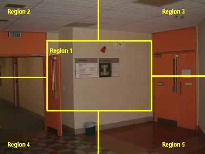
|
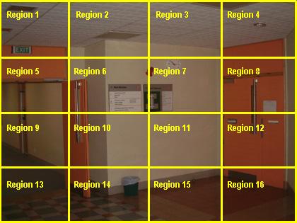
|
In the QBE case, the database images compared to the query have to be requantised by finding for every pixel the closest colour in the query codebook. Then the colour histogram of the image in question can be matched to the query histogram.
The (dis)similarity of two images described by normalised colour histograms, h and h', is measured by computing a distance between the histograms in the colour space. The chosen metric effects both effectiveness and computational complexity of retrieval. The effectiveness indicates to which extent the quantitative similarity match the perceptual, subjective one.
In the simplest case, the distance is based on the Minkowski metrics, such as the city-block (L1 norm, or sum of absolute differences) or Euclidean distance (L2 norm, or sum of squared differences) between the relative frequencies of the corresponding colours, or on the histogram intersection proposed by Swain and Ballard:
It is easily shown that the Swain-Ballard intersection measure actually coincides with the absolute (city-block) distance:
The three above metrics comparing only the corresponding colour components between the histograms take no account of cross-relations of the different colour clusters. Thus the images with similar but not identical representative colours can be considered as dissimilar on the basis of the distance between the colour histograms. Quadratic-form metrics avoid this drawback by pairwise comparisons of all the component pairs:
where A = [aij] is the positive definite symmetric matrix K × K with components aij = aji specifying the dissimilarity between the code words ci and cj for the histogram components with indices i and j. To decrease the computational complexity of the quadratic-form metrics, only most significant components may be taken into account.
A special case of the quadratic-form metric is the Mahalanobis distance in which the dissimilarity matrix A is obtained by inverting the covariance matrix for a training set of colour histograms. Alternatively, the Mahalanobis distance can account for the covariance matrix of colours in a set of training images (then the colours that are dominant across all images and do not discriminate among different images will not effect the distance, as it should be). In the special case of uncorrelated histogram components when the covariance matrix is diagonal, the Mahalanobis distance reduces to a weighted Euclidean one. The weight of each squared difference of the histograms' components is inversely proportional to the variance of these components treated as random variables.
Core colour descriptors of the MPEG-7 standard exploit histogram analysis:
A generic colour histogram captures the colour distribution with reasonable accuracy for image search and retrieval but has too many independent characteristics to choose (e.g. a colour space, quantisation in that space, and quantisation of the histogram values). To ensure the interoperability between descriptors generated by different MPEG-7 systems, the set of histogram-based descriptors is limited to the scalable colour descriptor (SCD) and the colour structure descriptor (CSD). The SCD in the HSV colour space uses a Haar transform encoding to facilitate a scalable representation of the description and complexity scalability for feature extraction and matching. This descriptor can be used also for a collection of pictures or a group of frames, and the group of frames / group of pictures descriptor (GoP) specifies how to build such a histogram. The colour structure histogram in the HMMD colour space identifies local colour distributions using a small structuring window (Manjunath e.a., 2001).
The SCD achieves full interoperability between different resolutions of the colour representation, from 16 bits per histogram to around 1000 bits per histogram. The descriptor exploits the HSV colour space uniformly quantised to 16, 32, 64, 128, or 256 bins. The histogram values are truncated into an 11-bit integer representation. Different configurations of the SCD correspond to different partitioning of the HSV colour space:
| HSV bins | 16 | 32 | 64 | 128 | 256 |
|---|---|---|---|---|---|
| H levels | 4 | 8 | 8 | 8 | 16 |
| S levels | 2 | 2 | 2 | 4 | 4 |
| V levels | 2 | 2 | 4 | 4 | 4 |
For a more efficient encoding, the 11-bit integer values are nonlinearly mapped into 4-bit representation to give higher significance to small values with higher probability. This 4-bit representation of the 256-bin HSV histogram yields 1024 bits per histogram. To reduce this number and ensure scalability, the histogram is encoded with a Haar transform. The basic Haar transform unit converts two input values b1 and b2 into their sum, b1 + b2, and difference, b2 − b2, considered as primitive low- and high-pass filters, respectively. The idea behind the Haar encoding is that the number of bins halves after summing adjacent pairs in an initial histogram, so that the repetitive Haar transform forms histograms of 128, 64, 32, and so on bins from an initial 256-bin histogram. The difference Haar transform coefficients keep the information about finer-resolution histograms with higher number of bins. Typically, the differences between adjacent bins are small; thus the sign-alternate high-pass coefficients can be truncated to integer representation with only a small number of bits. The sign bit is always retained whereas the least significant bits of the magnitude part can be skipped. The sign-bit only representation (1 bit per coefficient) is extremely compact while retains good retrieval efficiency (Manjunath e.a., 2001). At the highest accuracy level, the magnitude part is represented with 1 - 8 bits depending on the relevance of the respective coefficients.
Similarity matching of the SCD histograms using the absolute (city-block) distance typically gives good retrieval accuracy. The same matching can be used for the Haar transform coefficients (but the results are not identical). The latter matching has the same complexity as the histogram matching (assuming the number of coefficients is equal to the number of histogram bins and the distance measure is the same). The computation of the Haar coefficients is simple and adds nothing to the feature extraction / matching complexity.
Different-size SCD representations are easily compared by matching subsets of Haar coefficients corresponding to a coarser approximation of the initial histogram. The same procedure allows for fast coarse-to-fine matching when, for a given query, a coarse SCD representation is matched first to select a subset of image candidates in a database, and then the refined matching with more coefficients is applied to only this subset.
The GoP descriptor extends the SCD to a collection of images, video segments, or moving regions. The joint colour histograms for the whole collection are formed from the individual histograms for its items by averaging, median filtering, and histogram intersection. The joint colour histogram is then encoded using the Haar transform just as in the SCD.
The CSD is defined with four variants of non-uniform quantisation of the HMMD colour space resulting in 184, 120, 64, and 32 bins, respectively. The quantisation divides the whole colour space into five (for the 184 bins) or four (otherwise) subspaces on the "difference" (i.e. max{R,G,B}−min{R,G,B}) component. The overall colour quantisation is obtained by uniform quantisation of the respective subspaces with the different number of quantisation levels for hue and intensity (0.5(max{R,G,B} + min{R,G,B}) values:
| Component | Subspace | Number of quantisation levels for K CSD bins | |||
|---|---|---|---|---|---|
| K=184 | 120 | 64 | 32 | ||
| Hue | 0 | 1 | 1 | 1 | 1 |
| 1 | 8 | 4 | 4 | 4 | |
| 2 | 12 | 12 | 6 | 3 | |
| 3 | 12 | 12 | 4 | 2 | |
| 4 | 24 | ||||
| Intensity | 0 | 8 | 8 | 8 | 8 |
| 1 | 4 | 4 | 4 | 2 | |
| 2 | 4 | 4 | 4 | 4 | |
| 3 | 4 | 4 | 4 | 2 | |
| 4 | 2 | ||||
Colour structure descriptors with 120, 64, or 32 bins to approximate the 184-bin CSD are obtained from the latter by re-quantising the colour represented by each bin of the 184-bin descriptor into the more coarsely quantised colour space specified in the above table.
The total number of samples in the structuring element is fixed at 64, but its spatial extent E×E, or equivalently the subsampling factor S depends on the image size, i.e. height H and width W as follows: E=8S and S=2p where p = max{0, integer(0.5log2WH−8)} and "integer(z)" denotes the closest integer to z. If the image size is less than 216, e.g. 256×256 or 320×240, then p = 0 and an 8×8 element with no subsampling is used. Otherwise the element's size grows up and only 64 equispaced elements are used to compute the histogram (e.g. p = 1, S = 2, and E = 16 for an image of size 640×480, and every alternate sample along the rows ans columns is then used). The origin of the structuring element is in its top-left sample. The locations of the structuring element over which the CSD is accumulated is given by the grid of pixels of the possibly subsampled input image.
The colour clustering minimises the weighted scatter, or distortion Di in each cluster Ci using the algorithm similar to K-means clustering:
where wx,y denotes a perceptual weight for the pixel (x,y); ci is the centroid of the cluster Ci, and cx,y is the colour vector for the pixel (x,y). The specific perceptual weights depend on the local pixel statistics to take into account higher sensitivity of human visual perception to changes in uniform (smooth) than in textured regions. Each cluster is characterised with its centroid (representative colour) and optionally with the variance of the colour vectors for the pixels associated with this cluster.
The spatial coherency of a given dominant colour is measured with the normalised average number of connected pixels of this colour (it is computed using a 3×3 mask). The overall spatial coherency is a linear combination of the individual spatial coherencies weighted with the corresponding percentages pi.
The dissimilarity between the two descriptors DCD1 = {(c1i, p1i, v1i) : i=1,...,n1}, s1} and DCD2 = {(c2i, p2i, v2i): i=1,...,n2}, s2}, if one ignores the optional variance and coherency parameter, is given with the distance equivalent to the quadratic distance for comparing two colour histograms:
Here, the coefficient aξ,η that specifies the similarity of two colours, cξ and cη depends on the Euclidean distance dξ,η = ||cξ−cη|| between these colours and the maximum distance dsim below which the two colours are considered similar. Any two dominant colours from a single description are separated with at least such a distance. In the CIE-Luv colour space for α between 1.0 and 1.5, a normal value for dsim is between 10 - 20.
The dominant color descriptor has 3 bits to represent the number of dominant colours and 5 bits for each of the percentage values uniformly quantised in the range [0, 1]. The colour space quantisation is not constrained by the descriptor. The optional colour variances are non-uniformly quantised to 3 bits per colour (equivalent to 1 bit per colour space component), and the spatial coherency is represented with 5 bits (0, 1, and 31 mean that it is not computed, no coherency, and highest coherency, respectively).
The CLD uses representative colours on an 8×8 grid followed by a discrete cosine transform (DCT) and encoding of the resulting coefficients (Manjunath e.a., 2001). First, an input image is divided into 64 (8×8) blocks in order to derive their average colours in the YCrCg colour space. Then the average colours are transformed into a series of 8×8 DCT coefficients (independently for Y, Cr, and Cg components), and a few low-frequency coefficients are selected using zigzag scanning and quantisation: CLD = {(ΨY,i, ΨCr,i, ΨCg,i): i = 1, ..., ν} where &Psi...,i denotes the i-th DCT coefficient of the corresponding colour component and the number ν of the coefficients generally is different for each component.
For matching two CLDs, the following dissimilarity measure is used:
where the larger weights w... are given to the lower frequency coefficients. The CLD has 63 bits as the default recommendation: six Y coefficients and three each of Cr and Cg coefficients. The zero-frequency DCT coefficients are quantised to 6 bits and the remaining to 5 bits each.
The colour information for CBIR is also represented with colour moments, colour sets, colour coherence vectors, or colour correlograms.
Here, q denotes the colour component (e.g., R, G, B or H, S, V) and S =2, 3, ..., is the order of the moment. The similarity between the moments is measured usually by the Euclidean distance.
However, if two images have only a similar subregion, their corresponding moments, as well as colour histograms, will be different, and the overall similarity measure will be low. This is why in many experimental QBE-oriented CBIR systems the images are split onto a fixed or adaptive set of regions, and the colour features of one query region are compared to all the regions of every image in question.
Because the features for one query region can be similar to those for other regions, the same vector quantisation that had been efficient for building the colour codebooks can also be applied for selecting the most informative vectors of the colour features. Typically, the centres of the clusters of the feature vectors serve as such colour primitives describing the query image.
In the WebSEEk, the colour HSI space is divided into 166 colours as follows. The space is considered as a cylinder with the axis representing the value (intensity) that ranges from pure black to pure white. The distance (radius) to the axis gives the saturation, or relative amount of presense of a colour, and the angle around the axis is the hue giving the chroma (tint, ot tone). The hue is represented with the finest resolution by a circular quantisation of the hue circle into 18 sectors (6 per each primary colour). Other colour components are represented with the coarser resolution by quantising each into three levels. In addition, the colourless greyscale signals are quantised into four levels. This gives in total 18 (H) × 3 (S) × 3 (I) + 4 (grey levels) = 166 disctinct colours.