|
"Texture - ...(in extended use) the constitution, structure, or
substance of anything with regard to its constituents or formative elements."
(The Oxford Dictionary, 1971; 1989).
"Texture - ...a basic scheme or structure; the overall structure of
something incorporating all of most of parts." (Webster's Dictionary, 1959; 1986).
|
Texture is a very general notion that can be attributed to almost everything
in nature. For a human, the texture relates mostly to a specific, spatially
repetitive (micro)structure of surfaces formed by repeating a particular
element or several elements in different relative spatial positions.
Generally, the repetition involves local variations of scale, orientation,
or other geometric and optical features of the elements.
Image textures are defined as images of natural textured surfaces and
artificially created visual patterns, which approach, within certain limits, these
natural objects. Image sensors yield additional geometric and optical
transformations of the perceived surfaces, and these transformations
should not affect a particular class of textures the surface belongs.
| 
| 
| 
|
| Flowers0001
| Flowers0002
| Leaves0011
| Metal0002
|
| 
| 
| 
|
| Synthesised textures
|
|
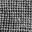
Examples of natural image textures (VisTex database, MIT Media Lab., USA) and
textures synthesised using a generic Gibbs random field (GGRF) model with multiple pairwise pixel
interactions.
|
It is almost impossible to describe textures in words, although each human
definition involves various informal qualitative structural features, such as
fineness - coarseness, smoothness, granularity, lineation, directionality,
roughness, regularity - randomness, and so on. These features, which
define a spatial arrangement of texture constituents, help to single out
the desired texture types, e.g. fine or coarse, close or loose, plain or
twilled or ribbed textile fabrics. It is difficult to use human classifications
as a basis for formal definitions of image textures, because there is no
obvious ways of associating these
features, easily perceived by human vision, with computational models that
have the goal to describe the textures. Nonetheless, after several decades
of reseach and development of texture analysis and synthesis, a variety of
computational characteristics and properties for indexing and retrieving
textures have been found. The textural features describe local
arrangements of image signals in the spatial domain or the domain of
Fourier or other spectral transforms. In many cases, the textural features
follow from a particular random field model of textured images
(Castelli & Bergman, 2002).
Many statistical texture features are based on co-occurrence
matrices representing second-order statistics of grey levels in pairs
of pixels in an image. The matrices are sufficient statistics of a Markov/Gibbs
random field with multiple pairwise pixel interactions.
A co-occurrence matrix shows how frequent is
every particular pair of grey levels in the pixel pairs, separated by a
certain distance d along a certain direction a.
Let g = (gx,y: x = 1, ..., M;
y = 1, ..., N) be a digital image. Let Q={0, ..., qmax}
be the set of grey levels. The co-occurrence matrix for a given inter-pixel
distance d and directional angle a is defined as
COOCm=d cos a, n=d sin a(g)=[COOCm, n(q, s|g):
q, s = 0, ..., qmax]
where COOCm, n(q, s|g) is the cardinality of the set
Cm,n of pixel pairs [(x,y), (x+m, y+n)]
such that gx,y=q and
gx+m,y+n=s.
Various statistical and information theoretic properties of the co-occurrence
matrices can serve as textural features (e.g., such features as homogeneity,
coarseness, or periodicity introduced by Haralick). But these features are
expensive to compute, and they were not very efficient for image classification and
retrieval (Castelli & Bergman, 2002).
Today's CBIR systems use in most cases
the set of six visual features, namely,
- coarseness,
- contrast,
- directionality,
- linelikeness,
- regularity,
- roughness
selected by Tamura, Mori, and Yamawaki
(Tamura e.a., 1977,
Castelli & Bergman, 2002) on the basis of psychological
experiments.
Coarseness relates to distances of notable
spatial variations of grey levels, that is, implicitly, to the size of the
primitive elements (texels) forming the texture. The proposed
computational procedure accounts for differences between the
average signals for the non-overlapping windows of
different size:
- At each pixel (x,y), compute six averages for the
windows of size 2k × 2k,
k=0,1,...,5, around the pixel.
- At each pixel, compute absolute differencesEk(x,y)
between the
pairs of nonoverlapping averages in the horizontal and
vertical directions.
- At each pixel, find the value of k that maximises the
difference Ek(x,y) in either direction and
set the best size Sbest(x,y)=2k.
- Compute the coarseness feature Fcrs by averaging
Sbest(x,y) over the entire image.
Instead of the average of Sbest(x,y, an improved
coarseness feature to deal with textures having multiple
coarseness properties is a histogram characterising the
whole distribution of the best sizes over the image
(Castelli & Bergman, 2002).
Contrast measures how grey levels q; q = 0, 1, ..., qmax,
vary in the image g and
to what extent their distribution is biased to black or white. The second-order
and normalised fourth-order central moments of the grey level histogram (empirical
probability distribution), that is,
the variance, σ2, and kurtosis, α4, are used
to define the contrast:
 where
where
 and m is the mean grey level, i.e. the first order moment
of the grey level probability distribution.
The value n=0.25 is recommended as the best for discriminating the
textures.
and m is the mean grey level, i.e. the first order moment
of the grey level probability distribution.
The value n=0.25 is recommended as the best for discriminating the
textures.
Degree of directionality is measured using the frequency
distribution of oriented local edges against their directional
angles. The edge strength e(x,y) and the
directional angle a(x,y) are computed using the
Sobel edge detector approximating the pixel-wise x- and
y-derivatives of the image:
| e(x,y) = 0.5(|Δx(x,y)| + |Δy(x,y)| )
|
| a(x,y) = tan-1(Δy(x,y) / Δx(x,y))
|
where Δx(x,y) and Δy(x,y) are the horizontal and
vertical grey level differences between the neighbouring pixels, respectively. The differences are
measured using the following 3 × 3 moving window operators:
| −1 | 0 | 1 | | 1 | 1 | 1
|
| −1 | 0 | 1 | | 0 | 0 | 0
|
| −1 | 0 | 1 | | −1 | −1 | −1
|
A histogram Hdir(a) of quantised direction values a is constructed
by counting numbers of the edge pixels with the corresponding directional
angles and the edge strength greater than a predefined threshold. The
histogram is relatively uniform for images without strong orientation and exhibits
peaks for highly directional images. The degree of directionality relates to the
sharpness of the peaks:
where np is the number of peaks, ap is the position
of the pth peak, wp is the range of the angles attributed to the
pth peak (that is, the range between valleys around the peak), r denotes a
normalising factor related to quantising levels of the angles a, and a is the
quantised directional angle (cyclically in modulo 180o).
Three other features
are highly correlated with the above three features and do not add much to the effectiveness
of the texture description. The linelikeness feature Flin
is defined as an average coincidence of
the edge directions (more precisely, coded directional angles) that co-occurred in the pairs of pixels separated by a
distance d along the edge direction in every pixel. The edge strength is expected
to be greater than a given threshold eliminating trivial "weak" edges. The coincidence is
measured by the cosine of difference between the angles, so that the co-occurrences in
the same direction are measured by +1 and those in the perpendicular directions by -1.
The regularity feature is defined as
Freg=1-r(scrs+scon+sdir + slin) where r is a normalising factor and each s...
means the standard deviation of the corresponding feature F... in each subimage
the texture is partitioned into. The roughness feature is given by simply summing the
coarseness and contrast measures:
Frgh=Fcrs+Fcon
In the most cases, only the first three Tamura's features are used for the CBIR. These
features capture the high-level perceptual attributes of a texture well and are useful for
image browsing. However, they are not very effective for finer texture discrimination
(Castelli & Bergman, 2002).
Random field models consider an image as a 2D array of random scalars (grey
values) or vectors (colours). In other words, the signal at each pixel location is a
random variable. Each type of textures is characterised by a joint probability
distribution of signals that accounts for spatial inter-dependence, or interaction
among the signals. The interacting pixel pairs are usually calles neighbours,
and a random field texture model is characterised by geometric structure and
quantitative strength of interactions among the neighbours.
If pixel interactions are assumed translation invariant, the interaction structure is
given by a set N of characteristic neighbours of each pixel. This results in
the Markov random field model where the
conditional probability of signals in each pixel (x,y) depends only on
the signals in the neighbourhood {(x+m,y+n): (m,n)
from the set N}.
In a special case of the simultaneous autoregressive (SAR)
Gauss-Markov model, the texture is represented by a set of parameters of the
autoregression:
Here, w is independent (white) noise with zero mean and unit variance, and
parameters a(m,n) and s specify the SAR model.
The basic problem is how to find the adequate neighbourhood, and this nontrivial
problem has no general solution.
More general generic Gibbs random field models with multiple
pairwise pixel interactions allow to relate the desired neighbourhood to a set of most
"energetic" pairs of the neighbours. Then the interaction structure itself and
relative frequency distributions of signal cooccurrences in the chosen pixel
pairs can serve as the texture features (Gimel'farb & Jain,
1996).
|
|
| MIT "Fabrics0008"
| Interaction structure
|
| with 35 neighbours
|
Texture features are usually compared on the basis of dissimilarity between the
two feature vectors. The dissimilarity is given by the Euclidean, Mahalanobis,
or city-block distance. In some cases, the weigted distances are used where
the weight of each vector component is inversely proportional to the standard
deviation of this feature in the database.
If the feature vector represents relative frequency distribution (e.g., a normalised
grey level cooccurrence histogram), the dissimilarity can also be measured by
the relative entropy, or Kullback-Leibler (K-L) divergence. Let
D(g,q) denote the divergence between two distributions,
fg = (fg,t :
t=1, ..., T) and fq = (fq,t :
t=1, ..., T). Then
This dissimilarity measure is asymmetric and does not represent a distance because the
triangle inequality is not satisfied. The symmetric distance is obtained by averaging
D(g,q) and D(q,g).
It should be noted that no single similarity measure achieves the best overall
performance for retrieval of different textures
(Castelli & Bergman, 2002).
If a texture is modelled as a sample of a 2D stationary random field,
the Wold decomposition can also be used for similarity-based retrieval
(Liu & Picard, 1996,
Castelli & Bergman, 2000). In the Wold model
a spatially homogeneous random field is decomposed into three mutually
orthogonal components, which approximately represent periodicity,
directionality, and a purely random part of the field.
The deterministic periodicity of the image is analysed using the autocorrelation
function. The corresponding Wold feature set consists of the frequencies
and the magnitudes of the harmonic spectral peaks (e.g., the K largest
peaks). The indeterministic (random) components of the image are modelled
with the multiresolution simultaneous autoregressive (MR-SAR) process. The
retrieval uses matching of the harmonic peaks and the distances between the
MRSAR parameters. The similarity measure involves a weighted ordering
based on the confidence in the query pattern regularity.
Experiments with some natural texture datrabases had shown that the Wold
model provides perceptually better quality retrieval than the MR-SAR model
or the Tamura's features (Castelli & Bergman, 2002).
An alternative to the spatial domain for computing the texture features is to use
domains of specific transforms, such as the discrete Fourier transform (DFT),
the discrete cosine transform (DCT), or the discrete wavelet transforms (DWT).
Global power spectra computed from the DFT have not been effective in texture
classification and retrieval, comparting to local features in small windows. At
present, most promising for texture retrieval are multiresolution features obtained
with orthogonal wavelet transforms or with Gabor filtering. The features describe
spatial distributions of oriented edges in the image at multiple scales.
A 2D Gabor function γ(x,y) and its Fourier transform
Γ(u,v) are as follows
(Manjunath & Ma, 1996):
where σu = 1/2πσx and
σv = 1/2πσy. The
Gabor function is a product of an elliptical Gaussian and a complex-plane wave
and it minimises joint 2D uncertainty in both spatial and frequency domain.
Appropriate
dilations and rotations of this function yield a class of self-similar Gabor filters
for orientation-
and scale-tunable edge and line detection. The filters
form a complete but non-orthogonal basis set for expanding an image
and getting its localised spatial frequency description. The total number of Gabor filters is
equal to the product of the numbers of scales and orientations.
A class of self-similar Gabor wavelets is produced from the "mother"
wavelet γ(x,y) by the dilations and rotations specified with the
generating function that depends on the integer parameters m and k and
the scale factor a > 1 as follows:
γmk(x,y) =
a−mγ(x′n,y′k)
where x′k =
a−m(x cos θk
+ y sin θk); y′k =
a−m(−x sin θk
+ y cos θk); &thetak =
kπ/K, and K is the total number of orientations.
The scale factor a−m for x′k
and y′k makes the filter energy independent of m.
To exclude sensitivity of the filters to absolute intensity values, the real (even)
components of the 2D Gabor filters are usually biased to make them zero mean. An
ensemble of grey-coded differently oriented odd (a) and even (b) 2D Gabor filters are
exemplified below (see Lee, 1996 for more detail):
These generalised
Gabor functions are of the following 2D form:
where (x0, y0) is the spatial location of the filter
centre in the image, and (u0, v0) is the spatial
frequency of the filter in the frequency domain.
The Gabor wavelets are not orthogonal. Therefore, to reduce the informational redundancy
of the filter outputs, the typical filter design strategy makes the
half-peak magnitude supports of the filter responses in the spatial frequency domain
touch each other. For example (Manjunath & Ma, 1996),
the contours below correspond to the half-peak magnitude of the
filter responses in the set of Gabor filters with the upper centre frequency
of interest, uh = 0.4, the lower centre frequency of interest,
ul = 0.05, six orientations (K = 6), and four scales
(S = 4):
In such a design, the scale factor a and filter parameters σu
and σv (and thus σx and σy)
are specified in terms of uh = W, ul,
K, and S, in
particular, a =
(uh/ul)−1/(S−1)
(Manjunath & Ma, 1996,
Vajihollahi & Farahbod, 2002):
The Gabor texture features include the mean and the standard deviation of the
magnitude of the Gabor wavelet transform coefficients. Given an image
g = (g(x,y): (x = 0, 1, ..., X−1;
y = 0, 1, ..., Y−1), the Gabor wavelet transform is
defined as
where the asterisk (*) indicates the complex conjugate, and the mean μmk
and the stabdard deviation σmk of the magnitude of the transformed image
describe each local texture region under an assumption of its spatial homogeneity:
A feature vector contains these pairs for all the scales and orientations of the wavelets,
e.g. for the six orientations (K = 6), and four scales (S = 4) the feature
vector contains 24 pairs:
f=(μ00, σ00, ...,
μ35, σ35).
The MPEG-7 multimedia content description interface
involves three texture descriptors for representing texture
regions in images
(Manjunath e.a., 2001; Sikora, 2001), namely,
- the texture browsing descriptor
to characterise perceptual directionality, regularity, and coarseness of a texture,
- the homogeneous texture descriptor (HTD) to quantitatively characterise
homogeneous texture regions for similarity retrieval using local spatial statistics
of the texture obtained by scale- and orientation-selective
Gabor filtering, and
- the local edge histogram descriptor to characterise non-homogeneous
texture regions.
This 12-bit descriptor relates to regularity, directionality, and coarseness (scale) of visual
texture perception and can be used both for browsing and coarse classification
of textures. First, the image is filtered with a bank of orientation- and scale-tuned
Gabor filters in order to select and code two dominant texture orientations (3 bits per
orientation). Then an analysis of filtered projections of the image along the dominant
orientations specify the regularity (2 bits) and coarseness (2 bits per scale).
The second dominant orientation and second scale features are optional.
The regularity of a texture has four levels, from 0 (irregular, or random
texture) to 3 (a periodic pattern). There is an ambiguity in the intermediate
two values: a well-defined directionality with no perceivable micro-pattern is
considered more regular than a pattern that lacks directionality and periodicity,
even if the individual micro-patterns are clearly identified:
| Texture regularity | 00 (irregular) | 01 | 10 | 11 (periodic)
|
|---|
Texture example
from the Brodatz's
digitised set
| 
| 
| 
| 
|
| D005 | D066 | D068 | D001
|
The directionality of a texture is quantified to six values from 0o to
150o in steps of 30o. In particular, the above texture D001
has strong vertical and horizontal directionalities. The descriptor specifies up to two
dominant directions encoded each to 3 bits: 0 means a texture does not have
any dominant directionality, and the remaining directions have values from 1 to 6.
The coarseness associated with each dominant direction relates to image
scale or resolution and is quantised to four levels: 0 indicates a fine grain
texture and 3 indicates a coarse texture. These values are also related to the
frequency space partitioning used in computing the HTD (see the next section).
To compute the browsing descriptor, an image is filtered using a bank of scale
and orientation selective band-pass filters similar to those for the HTD. The
filtered outputs are then used to compute the components of the texture browsing
descriptor. Bec ause the descroptor semantics relates to human perception of
the texture, the descriptor can be also specified manually. In browsing, any
combination of the three main components - regularity, directionality, and coarseness -
can be used to browse the database. In similarity retrieval, the texture browsing
detector can be used to select a set of candidates; then the HTD provides a precise
similarity matching among the candidate images.
Homogeneous texture is an important visual
primitive for searching and browsing through large collections of similar looking patterns.
If an image can be partitioned into a set of homogeneous texture regions, then the
texture features associated with the regions can index the image data. Examples of
homogeneous textured patterns are viewed from a distance
parking lots with cars parked at regular intervals, or
aagricultural areas and vegetation patches in aerial and satellite imagery.
Examples of queries that could be supported in this context could include
"Retrieve all satellite images with less than 20% cloud cover"
or "Find a vegetation patch that looks like this region"
(Martinez, 2004).
This descriptor uses 62 8-bit numbers per image or image region in order to
allow for accurate search and retrieval. The image is filtered with a bank of
orientation and scale sensitive Gabor filters,
and the means and the standard deviations of the
filtered outputs in the spatial frequency domain (5 scales × 6 orientations per scale)
are used as the descriptor components.
The frequency space is partitioned into 30 channels with equal angular
divisions at 30o intervals and five-octave division in the radial
direction:
In a normalised frequency space 0 ≥ &omega ≥ 1, the centre frequencies of the
feature channels are spaced equally in 30o in angular direction such that
the polar angle θk = 30ok where k
= 0, 1, ..., 5 is angular index. In the radial direction, the centre frequencies
of the neighbouring feature channels are spaced one octave apart:
ωm = 2−mω0 where
m = 0, 1, ..., 4 is radial index and ω0 = 0.75 is the highest
centre frequency, i.e. ω1 = 0.375; ω2 = 0.1875;
ω3 = 0.09375, and ω4 = 0.046875. The octave
bandwidths Bm are, respectively, B0 = 0.5;
B1 = 0.25;
B2 = 0.125; B3 = 0.0625,
and B4 = 0.03125.
The channel index i = 6m + k + 1.
The Gabor filters for the feature channels are represented in the polar coordinates;
the Fourier transform of such a 2D Gabor function is:
The filter parameters ensure that the half-peak contours of the 2D Gaussians of adjacent
filters in the radial and angular directions touch each other:
σθ,k = 15o/(2 ln 2)0.5 and
σω,m = 0.5Bm/(2 ln 2)0.5.
The mean and standard deviation of the filter output are logarithmically scaled
to obtain two numerical features (ei and di,
respectively) for each channel i. In addition to these 2×30 = 60 features,
the HTD includes also the mean
intensity fDC and the standard deviation fSD of the image:
HTD = [fDC, fSD, e1, ...,
e30, d1, ..., d30].
The edge histogram descriptor resembles the colour layout descriptor (CLD) in its
principle of capturing the spatial distribution of edges which is useful in image matching
even if the texture itself is not homogeneous. An image is partitioned into 4×4 = 16
sub-images, and 5-bin local edge histograms are computed for these sub-images, each histogram
representing five broad categories of vertical, horizontal, 45o-diagonal,
135o-diagonal, and isotropic (non-orientation specific) edges. The resulting
scale-invariant descriptor is of size 240 bits, i.e.16×5 = 80 bins and supports
both rotation-sensitive and rotation-invariant matching
(Manjunath e.a., 2001; Sikora, 2001).
The edge histograms are computed by subdividing each of the 16 sub-images into a fixed
number of blocks. The size of these blocks depends on the image size and is assumed to be
a poer of 2. To have the constant number of blocks per sub-image, their sizes are scaled
in accord with the original image dimensions. Each block is then treated as 2×2 pixel
image (by averaging each of the 2×2 partitions), and a simple edge detector is
applied to these average values. The detector consists of four directional filters and
one isotropic filter:
Five edge strengths, one for each of the five filters, are computed for each image block.
If the maximum of these strengths exceeds a certain preset threshold, the corresponding
image block is an edge block contributing to the edge histogram bins. The bin values are
normalised to the range [0.0, 1.0] and non-linearly quantised into 3 bits per bin.
-
V. Castelli and L. D. Bergman (Eds.). Image Databases: Search and
Retrieval of Digital Imagery. Wiley: New York, 2002.
-
G.L.Gimel'farb and A.K.Jain. On retrieving textured images from an image
data base. Pattern Recognition, vol. 29, no. 9, 1996, 1441 - 1483.
-
A.Hanjalic, G. C. Langelaar, P. M. B. van Roosmalen, J. Biemond,
and R. Lagendijk. Image and Video Data Bases: Restoration, Watermarking and Retrieval.
Elsevier Science: Amsterdam, 2000.
-
T. S. Lee. Image representation using 2D Gabor wavelets. IEEE Transactions on
Pattern Analysis and Machine Intelligence,
vol. 18, no. 10, 1996, 959 - 971.
-
F. Liu and R. W. Picard. Periodicity, directionality, and randomness:
Wold features for image modeling and retrieval. IEEE Transactions on Pattern Analysis
and Machine Intelligence, vol. 18, no. 7, 1996, 722 - 733.
-
B. S. Manjunath, J.-R. Ohm, V. V. Vasudevan, and A. Yamada. Color and texture
descriptors. IEEE Transactions on Circuits and Systems for Video Technology,
vol. 11, no. 6, 2001, 703 - 715.
-
B. S. Manjunath and W. Y. Ma. Texture features for browsing and retrieval
of image data. IEEE Transactions on Pattern Analysis and Machine Intelligence,
vol. 18, no. 8, 1996, 837 - 842.
-
J. M. Martinez, Ed. MPEG-7 Overview. ISO/IEC JTC1/SC29/WG11 No. 6828 (2004).
On-line.
http://www.chiariglione.org/mpeg/standards/mpeg-7/mpeg-7.htm#E12E27
-
S. M. Rahman (Ed.). Interactive Multimedia Systems.
IRM Press: Hershey, 2002.
-
T. K. Shih. Distributed Multimedia Databases: Techniques &
Applications. Idea Group Publishing: Hershey, 2002.
-
T. Sikora. The MPEG-7 visual standard for content description - an
overview. IEEE Transactions on Circuits and Systems for Video Technology,
vol. 11, no. 6, 2001, 696 - 702.
-
A. W. M. Smeulders and R. Jain (Eds.). Image Databases and
Multimedia Search. World Scientific: Singapore, 1997.
-
H. Tamura, S. Mori, and T. Yamawaki. Texture features
corresponding to visual perception. IEEE Transactions on Systems, Man, and
Cybernetics, vol. SMC-8, no. 6, 1978, 460 - 473.
-
M. Vajihollahi and R. Farahbod.
The MPEG-7: Visual Standard for Content Description, 2002. On-line:
http://www.cs.sfu.ca/CC/820/li/material/presentations/paper8.ppt
Return to the local table of contents
Return to the general table of contents