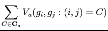
The partial energy
![]() in
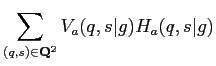
Eq. (6.1.1) can be factorised into a product
of a potential vector and a vector representing marginal probability
distribution of signal co-occurrences
in
Eq. (6.1.1) can be factorised into a product
of a potential vector and a vector representing marginal probability
distribution of signal co-occurrences
![]() at the
pixel pairs.
at the
pixel pairs.
Here,
![]() denotes the empirical marginal probability
distribution of the pixel pair
denotes the empirical marginal probability
distribution of the pixel pair
![]() separated by
the displacement vector of the clique family
separated by
the displacement vector of the clique family
![]() .
.
![]() represents the grey level co-occurrence histogram (GLCH) collected
over the image
represents the grey level co-occurrence histogram (GLCH) collected
over the image ![]() for the clique family
for the clique family
![]() , and
, and
![]() is
the normalised GLCH. The potential component
is
the normalised GLCH. The potential component ![]() represents
the strength of interaction between grey levels
represents
the strength of interaction between grey levels ![]() and
and ![]() over the
clique family
over the
clique family
![]() .
.
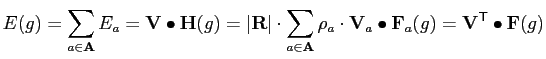
By Eq. (6.2.3), the total energy ![]() in
Eq. (6.1.3) can be rewritten as follows,
in
Eq. (6.1.3) can be rewritten as follows,
Here,
![]() ,
,
![]() ,
,
![]() and
and
![]() denote the potential vector, the weighted potential
vector, the GLCH vector and the normalised GLCH vector,
respectively, and
denote the potential vector, the weighted potential
vector, the GLCH vector and the normalised GLCH vector,
respectively, and
![]() denotes the
weight or the relative cardinality of the clique family
denotes the
weight or the relative cardinality of the clique family
![]() .
.
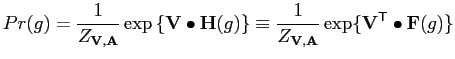
After substituting the energy ![]() of
Eq. (6.2.4) into
Eq. (6.1.3), a generic MGRF model is
specified by the following distribution,
of
Eq. (6.2.4) into
Eq. (6.1.3), a generic MGRF model is
specified by the following distribution,
Eq. (6.2.5) reveals a few important statistical
properties of a generic MGRF model. First, the Gibbs distribution
belongs to the exponential families [2] of
probability distributions and therefore to the MaxEnt distributions.
The exponential part of the distribution is a linear combination of
the potential vector
![]() and the GLCH vector
and the GLCH vector
![]() . The maximum entropy properties of the exponential
families are well known in applied and theoretical
statistics [2], well before the MaxEnt principle was
reintroduced into texture modelling in [113]. Second, the
potential vector
. The maximum entropy properties of the exponential
families are well known in applied and theoretical
statistics [2], well before the MaxEnt principle was
reintroduced into texture modelling in [113]. Second, the
potential vector
![]() are the model parameters to
be estimated, while the GLCH vector
are the model parameters to
be estimated, while the GLCH vector
![]() are the sufficient
statistics to the model.
are the sufficient
statistics to the model.
The GPD function for a generic MGRF model in
Eq. (6.2.5) is very similar to that of the FRAME model
in Eq. (5.2.25), except that two models involve different
sufficient statistics. The FRAME model is derived from GLHs
collected from responses of a filter bank, but a generic MGRF model
uses the GLCH statistics. If each signal pair
![]() is considered as the output
of a local 'filter', then the grey level co-occurrences histogram in
a generic MGRF model could be considered a joint distribution of
filter responses. Hence, a generic MGRF and the FRAME models are
equivalent in this sense.
is considered as the output
of a local 'filter', then the grey level co-occurrences histogram in
a generic MGRF model could be considered a joint distribution of
filter responses. Hence, a generic MGRF and the FRAME models are
equivalent in this sense.
For both models, identifying an optimal set of characteristic statistics for a training image is a key issue for successful modelling an image. Too big number of statistics involved in a model ultimately lead to intractable complexity of model identification, while insufficient statistics lead to inadequate modelling. In a generic MGRF model, an analytic first approximation of potentials is computed for ranking and selecting the most characteristic clique families, and the GLCHs for selected families act as sufficient statistics of the model. In the FRAME model, identifying sufficient statistics involves a stepwise procedure of filter selection from a predefined filter bank [113]. The procedure is conceptually similar to the method for sequential selection of clique families for an MGRF model [107], i.e. the filter selected at each step maximises the change of the related marginal distribution. A major deficiency of this approach is that the initial filter bank has to be constructed heuristically which might not contain all `important' filters to the image.