| 
|
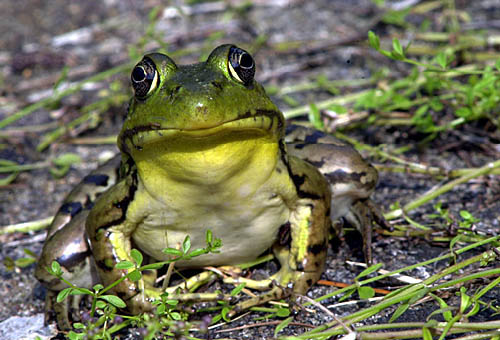
Image geometry appears in the form of spatial relationships between the pixels or
groups of pixels. Geometric operations change these relationships by moving pixels to new
locations while preserving to some extent pixel neighborhoods:
|
|
|
Geometric transformations are necessary if the imaging process suffers from some
inherent geometric distortions. For instance, a high-resolution airborne line scanner, which
sweeps each sensor across the terrain below (so called "pushbroom imaging")
produces extremely distorted images due to changes in velocity, altitude, and attitude, i.e.
yaw, pitch, and swing angles of the aircraft during the image acquisition:
Even if an image has no geometric distortion, its geometry may need some modification, e.g. to adjust an image of the Earth's surface to a certain map projection or to register two or more images of the same scene or object, acquired with different imaging devices or obtained from different viewpoints. Image registration pursues the goal of bringing common features in two or more images into coincidence.
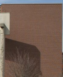
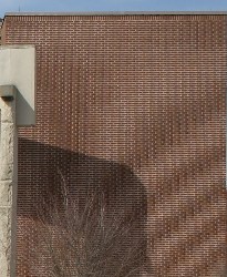
Simple techniques for manipulating image geometry such as replication of each pixel to an
n×n block of pixels to enlarge an image or subsampling (taking one pixel from
each n×n block) to shrink an image have serious limitations due to information
losses and Moire effects of subsampling as well as
"blocky" appearance of images enlarged by pixel
replication. The limitations become
obvious when a subsampled image is enlarged to its previous size by simply replicating the
sampled pixels - see, e.g. below the original and subsampled/enlarged images taken from
http://www.robots.ox.ac.uk/~improofs/super-resolution/super-res1.html, or
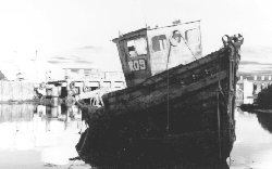
the aliasing due to the inadequate sampling resolution,
or pixel density, which appears
as a Moire pattern (the latter image pair is borrowed from from Wikipedia
http://en.wikipedia.org/wiki/Nyquist-Shannon_sampling_theorem):
| 
| 
| 
|
| Information losses due to subsampling and subsequent block enenlargement | Aliasing due to the inadequate sampling resolution | ||
An arbitrary geometric transformation moves a pixel at coordinates (x,y) to a
new position, (x′,y′). The movement is specified by a pair of
transformation equations:
| 
|
| Initial image | Affinely transformed image |
| Transformation | a0 | a1 | a2 | b0 | b1 | b2 |
|---|---|---|---|---|---|---|
| Translation by (Δx,Δy) | 1 | 0 | Δx | 0 | 1 | Δy |
| Uniform scaling by a factor s | s | 0 | 0 | 0 | s | 0 |
| Non-uniform scaling by factors sx, sy | sx | 0 | 0 | 0 | sy | 0 |
| Clockwise rotation through angle θ | cos θ | sin θ | 0 | −sin θ | cos θ | 0 |
| Horizontal shear by a factor h | 1 | h | 0 | 0 | 1 | 0 |
An identity transformation with Δx=Δy=h=0; s=sx=sy=1, θ=0, i.e. a0=b1=1 and zero-valued other coefficients, does not change pixel positions. Given an arbitrary transformation T, an inverse transformation T−1 returns every transformed point to its initial position.
Combinations of translations and rotations only form so-called Euclidean transformations that preserve angles between lines and distances between points.
Because any combination of these special cases is also an affine transformation,
any arbitrary affine transformation is usually expressed as some combination of these
simpler processing steps, performed in sequence. Generally, such a sequence is more
meaningful than direct specification of the transformation matrix: e.g. the four
sequential steps of (i) horizontal shear by the factor 0.5, (ii) clockwise
rotation through the
angle θ = −53o.13 (so that cos θ = 0.6 and sin θ = −0.8),
i.e. counterclockwise rotation through the angle 53o.13,
(iii) uniform scaling by the factor 2, and (iv) translation by (3,−2)
result in the following affine transformation matrix in homogeneous coordinates:
|
|
Any geometric transformation, including an affine transformation, can be implemented as forward or backward mapping. The forward mapping iterates over each pixel of the input image, computes new coordinates for it, and copies its value to the new location. But the new coordinates may not lie within the bounds of the output image and may not be integers. The former problem is easily solved by checking the computed coordinates before copying pixel values. The second problem is solved by assigning the nearest integers to x′ and y′ and using these as the output coordinates of the transformed pixel. The problem is that each output pixel may be addressed several times or not at all (the latter case leads to "holes" where no value is assigned to a pixel in the output image).
The backward mapping iterates over each pixel of the output image and uses the inverse transformation to determine the position in the input image from which a value must be sampled. In this case the determined positions also may not lie within the bounds of the input image and may not be integers. But the output image has no holes.
Any interpolation scheme convolves image data with an interpolation function giving grey levels for real-valued positions in an image.
Zero-order interpolation, or nearest-neighbour interpolation rounds real-valued coordinates calculated by a geometric transformation to their nearest integers. Let x = Tx(x′,y′) and y = Ty(x′,y′) be real coordinates of a point in the input image calculated with an inverse transformation T for backward mapping of the integer output position (x′,y′). Then the nearest-neighbour interpolation copied to the latter position the value in the integer position (xzo = ⌈x−0.5⌉, yzo = ⌈y−0.5⌉) where ⌈z⌉ denotes the integer upper bound of z, i.e. the minimum integer greater than or equal to z. The corresponding 1D interpolation function is: h(z) = 1 if −0.5 ≤ z ≤ 0.5 and 0 otherwise, and the 2D interpolation finction h(x,y) is specified a separable product h(x,y) = h(x)h(y).
Zero-order interpolation is simple computationally but input linear elements may become degraded in a transformed image, and the latter is too "blocky" after being scaled up in size by a large factor due to a discontinuous zero-order interpolation function.
First-order interpolation, or bilinear interpolation produces better
visual appearance of the transformed image. An output pixel grey level is computed as
a hyperbolic distance-weighted function of the four pixels in integer positions
(x0,y0),
(x1,y0),
(x0,y1), and
(x1,y1),
surrounding the calculated real-valued position (x,y).
Here, x1 = ⌈x⌉;
y1 = ⌈y⌉;
x0 = x1 − 1, and
y0 = y1 − 1.
Let fαβ = f(xα,yβ);
α,β∈[0,1], be grey levels in the surrounding pixels. Let
(Δx = x - x0,
Δy = y - y0) denote the real-valued
translation of the transformed position with respect to its integer rounding.
Then first-order
interpolation function is as follows:
More visually appealing but far more complex computationally third-order interpolation, or bicubic interpolation convolves a 16×16 pixel neighbourhood with a continuous cubic function having a continuous derivative.
The transformation equations mapping (x,y) to (x′,y′)
are generally expressed as polynomials in x and y, e.g. a quadratic
warp with 12 coefficients
In a piecewise warping, a control grid on the input image guides the warping.
The grid, being a mesh of horizontal and vertical lines, covers the entire image with
a set of quadrilaterals (rectangles). The
intersections of the grid lines are control points being moved to new positions
in the output (transformed) image. After the piecewise warping, every quadrilateral in the
initial grid maps onto a quadrilateral in the warped grid. To uniquely determine
the mapping, an 8-parameter bilinear transformation similar to the affine
transformation but with an extra term in xy is used:
Morphing is an incremental transformation of one image into another. It combines the ideas of piecewise warping / registration and is used mostly for special TV, movie, or presentation effects rather than in image processing. At each step, a certain mesh is mapped into a transformed one, using an affine transformation to relate one triangle of the initial triangular mesh to the corresponding triangle of the goal mesh, or a bilinear transformation for the quadrilateral meshes. The basic difference from the piecewise warping is that the morphing computes the overall warp incrementally, as a sequence of smaller warps.
These lecture notes follow Chapter 9 "Geometric Operations" of the textbook