


Some useful Internet links:
Stereo vision infers spatial structure and 3D distances of visible points
of a scene from two or more images taken from different viewpoints:

| 
| 
| 
| |
| Left and right images of a horizontal stereo pair | Left and right images of a horizontal stereo pair | |||
In so doing, a stereo system acquires stereo images, determines which points of the images correspond to, i.e. are projections of the same scene point (the correspondence problem), and reconstructs the 3D location and structure of the observed objects from a number of corresponding points and available information on the geometry of stereo acquisition (the reconstruction problem). To solve the correspondence problem means to determine which parts of the stereo images, i.e. of the left and right images of a stereo pair represent the same scene element. To solve the reconstruction problem means that observed 3D surfaces are determined from the corresponding parts of the images and the known geometry of image acquisition.
Disparity,
or difference in image position between corresponding points relates to
3D location of the scene point. The disparities of all the image points
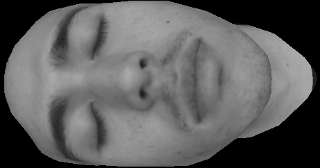
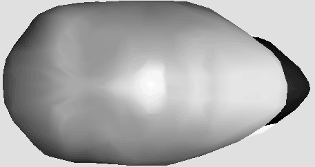
form the so-called disparity map that can be displayed as an image
using greyscale coding of the disparities. If the geometry of image
acquisition is known, the disparity map can be converted into a 3D
map of the viewed scene:
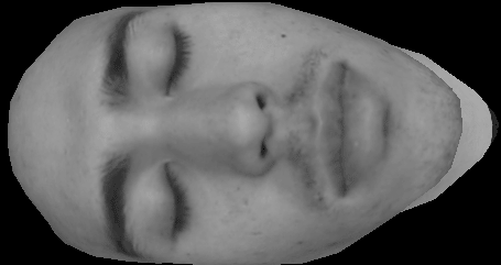
| 
| 
|
| Upper image of a vertical stereo pair | Bottom image of a vertical stereo pair | Disparity map |
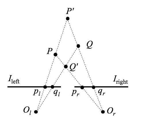
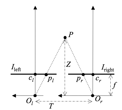
A simple stereo system below consists of two pinhole cameras with the coplanar
image planes and parallel optical axes:
| 
| |
| 3D reconstruction depends on the solution of the correspondence problem | Depth is evaluated from the disparity of the corresponding points |
The left and right image planes are represented by the segments Ileft and Iright respectively, and Ol and Or are the centres of projection, or optical centres of the cameras. Because the optical axes are parallel, their point of intersection called the fixation point lies intinitely far from the cameras. Generally, stereo systems may have verging optical axes, with the fixation point at a finite distance from the cameras.
The position of an observed spatial point, e.g. P in the above figure, is determined by triangulation, i.e. by interesecting the backtracing rays from the images, pl and pr, of P formed by the two cameras through the centres of projection. If (pl, pr) is a pair of corresponding points, interesecting the rays plOl and prOr gives the spatial point P having projections pl and pr. Triangulation depends crucially on which pairs of image points are cosen as corresponding points. In the above figure, triangulation of the corresponding pairs (pl, pr) and (ql, qr) leads to interpreting the image points as projections of P and Q, respectively; but triangulation of the corresponding pairs (pl, qr) and (ql, pr) returns P′ and Q′. Both interpretations are totally different but equally justified once the respective correspondences are accepted.
Triangulation in the above simple stereo system reconstructs the 3D position of each single
observed point P from its projections, pl and pr,
using the known distance, T, between the centres of projection
Ol and Or and the common focal length, f, of
the cameras. The distance T is called the baseline of the
stereo system. Let (xl, y) and (xr, y)
be the 2D coordinates of the image points pl and pr
with respect to the principal points (traces of the optical axes) cl
and cr as the origins of (x,y)-image coordinates, the
x-axis being parallel to the baseline. The 3D (X,Y,Z)-coordinate
frame has the distance (depth) Z-axis parallel to the optical axes, the
X-axis parallel to the baseline and the image x-axes , and the
Y-axis parallel to the image y-axes. Assuming the 3D coordinate
frame has the origin in the optical centre of the left camera, the image
coordinates of the spatial point P = (XP,YP,ZP)
are as follows:
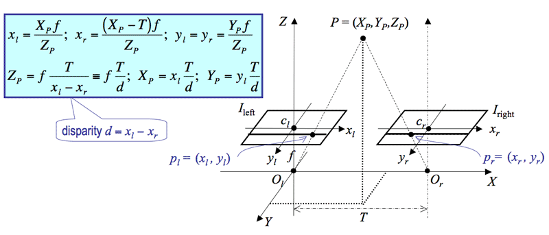
The disparity d measures the difference in image position between the corresponding
points in the two images. The depth is inversely proportional to disparity, the infinitely
far points (i.e. ZP = ∞) having zero disparity in this simple stereo
system.
Return to the table of contents
These lecture notes follow Chapter 7 "Stereopsis" of the textbook of E. Trucco and A. Verri, "Introductory Techniques for 3-D Computer Vision", Prentice Hall, NJ, 1998, with extra examples and materials taken mostly from the Web (with corresponding references) and from the following publications:
Return to the table of contents
If A is real-valued and symmetric n×n matrix, Aij = Aji, it has N linearly independent (or mutually orthogonal) eigenvectors e1, e2, …, en. Typically, the eigenvectors are normalised so that their dot product ei•ej = 1 if i=j and 0 otherwise. Such eigenvectors are called orthonormal.
Each eigenvector en has its own eigenvalue λn such that
Aei = λiei. For example, let A be an arbitrary
2×2 symmetric real matrix with the components a, b, c:
 .
.
Then its eigenvalues are the two solutions of the above quadratic equation:
 .
.
For example, if a = c = 1 and b = 0 (the 2×2 identity matrix),
then both the eigenvalues are equal to 1:
 .
.
Actually, in this case the matrix equations Ae = λe themselves do
not constrain the eigenvectors (they give only the identities
ej,i = ej,i for i,j = 1, 2), so that
only the constraints due to their orthonormality hold.
In this case there exist infinitely many possible pairs of eigenvectors of the following form:
e1 = [cos θ sin θ]T and
e2 = [−sin θ cos θ]T
where θ is an arbitrary angle, e.g. θ = 0 for the above pair
e1 = [1 0]T and
e2 = [0 1]T.
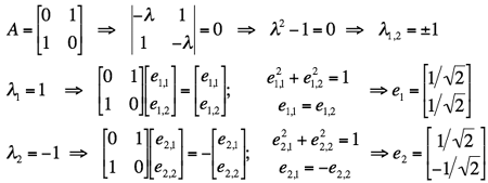
If a = c = 0 and b = 1, then λ1 = 1 and
λ2 = −1. The corresponding eigenvectors are obtained as follows:
 .
.
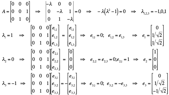
Two more examples of computing eigenvalues and eigenvectors for particular
3×3 symmetric real matrices:
 ,
,
and
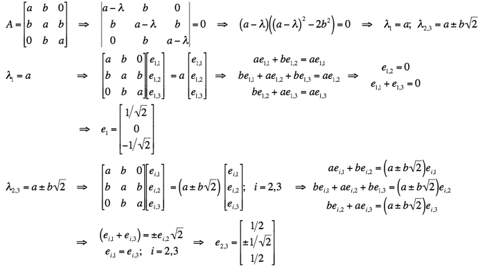 .
.
Additional information about eigenvalues and eigenvectors can be found in:
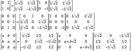
Matrix diagonalisation (called also eigendecomposition) is defined for a square n×n matrix A with N orthogonal eigenvectors such as a symmetric real one. Let E =[e1 e2 … en] be the n×n matrix with the orthonormal eigenvectors of A as the columns, i.e. Eij = ej,i. Then AE = [λ1e1 λ2e1 … λnen] is the matrix having as the columns the eigenvectors factored by their eigenvalues, i.e. the matrix with the components (AE)ij = λjej,i; i,j = 1, …, N, where ej,i is the i-th component of the j-th eigenvector.
In the transpose, ET, the same eigenvectors form the rows. Therefore, ETE = I, so that the matrix E is orthogonal, that is, its transpose, ET, is the (left) inverse, E−1.
Hence ETAE = Λ where Λ is the n×n diagonal matrix Λ = diag{λ1, λ2, …, λN} with the components &Lambdaij = λi if i=j and 0 otherwise. Because every real symmetric matrix A is diagonalised by the transformation ETAE = Λ, it is decomposed into a product of the orthogonal and diagonal matrices as follows: A = EΛET.
In particular,
 .
.
Additional information about eigendecomposition can be found in:
SVD is defined for a generic, rectangular matrix as follows: Any m×n matrix A can be written as the product of three matrices: A = UDVT. The columns of the m×m matrix U are mutually orthogonal unit vectors, as the columns of the n×n matrix V. The m×n matrix D is diagonal; its diagonal elements, σi, called singular values are such that σ1≥σ2≥ … ≥σN≥0. The matrices U and V are not unique, but the singular values are fully determined by the matrix A.
The SVD has the following properties:
 . It follows from the SVD
A = UDVT that
 .
.
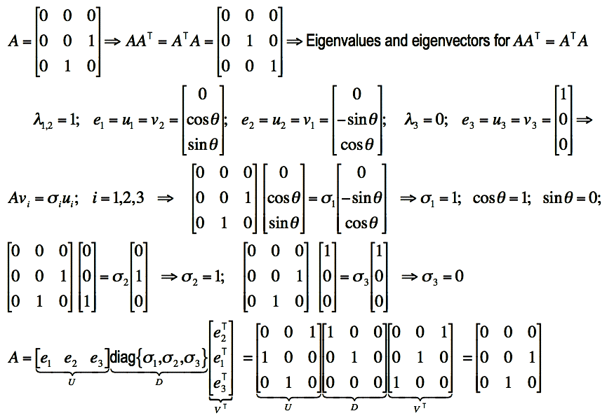
An example of the SVD of the symmetric singular square 3×3 matrix being used
earlier in the eigendecomposition is as follows
(in this particular case the matrices ATA
and AAT are the same, but their eigenvectors for the same
eigenvalues are used in different order
in U and V to ensure the non-negative singular values):
 .
.
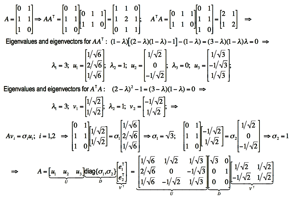
The next example presents the SVD of a simple 3×2 rectangular matrix:
 .
.
Note that there is another definition of SVD with the m×n matrix U and n×n matrices D and V which is typically used in computations (see e.g. W. H. Press, B. P. Flannery, S. A. Teukolsky, and W. T. Vetterling, Numerical Recipes in FORTRAN: The Art of Scientific Computing, Cambridge University Press, UK, 2nd ed., 1992: Section 2.6 "Singular Value Decomposition", pp. 51-63) because of a smaller memory space for the matrices: mn + 2N2 rather that m2 + mn + N2 for the initial definition as typically N << m. The latter SVD definition is used e.g. in the C-subroutine svd() being a very straighforward translation into C of the Fortran program developed in the Argonne National Laboratory, USA, in 1983.
Additional information about SVD can be found in:
Let an over-determined system of m linear equations, Ax = b, have to be solved for an unknown N-dimensional vector x. The m×n matrix A contains the coefficients of the equations, and the m-dimensional vector b contains the data. If not all the components of b are null, the optimal in the least square sense and the shortest-length solution x∗ of the system is given by x∗ = (ATA)+ ATb. The derivation is as follows:
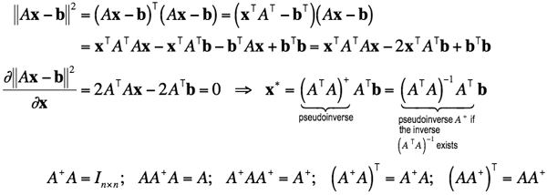 .
.
If the inverse of (ATA) exists, then the matrix A+ = (ATA)−1 AT is the pseudoinverse, or Moore-Penrose inverse. If there are more equations than unknowns, the pseudoinverse is more likely to coinside with the inverse of ATA, but it is better to compute the pseudoinverse of ATA through SVD to account for the condition number of this matrix.
While only a square full-rank matrix A has the conventional inverse A−1, the pseudoinverse A+ exists for any m × n matrix; m > n. Generally, SVD (singular value decomposition) is the most effective way of getting the pseudoinverse: if A = UDVT where the m×m matrix U and n×n matrix V are orthogonal and the m×n matrix D is diagonal with real, non-negative singular values σ1≥σ2≥ … ≥σN≥0, then A+ = V(DTD)−1 DTUT.
This and additional information about the pseudoinverse matrix can be found in:
Let one have to solve a homogeneous system of m linear equations in N unknowns, Ax = 0 with m≥n−1 and rank(A)=N−1. A nontrivial solution unique up to a scale factor is easily found through SVD: this solution is proportional to the eigenvector corresponding to the only zero eigenvalue of ATA (all other eigenvalues being strictly positive because the rank of A is equal to N−1). This is proved as follows. Since the solution may have an arbitrary norm, a solution of unit norm in the least square sense has to minimise the squared norm ||Ax||2 = (Ax)TAx = xTAT Ax, subject to the constraint xTx = 1. This is equivalent to minimise the Lagrangian L(x) = xTAT Ax − λ(xTx − 1). Equating to zero the derivative of the Lagrangian with respect to x gives ATAx − λx = 0, so that λ is an eigenvalue of the matrix ATA, and the solution, x = eλ, is the corresponding eigenvector. The solution makes the Lagrangian L(eλ) = λ; therefore, the minimum is reached at λ = 0, the least eigenvalue of ATA.
According to the properties of SVD, this solution could have been equivalently established as the column of V corresponding to the only null singular value of A (the kernel of A). This is why one need not distinguish between these two seemingly different solutions of the same problem.
Let entries of a matrix, A, to be estimated satisfy some algebraic constraints (e.g., A is an orthogonal or the fundamental matrix). Due to errors introduced by noise and numerical computations, the estimated matrix, say Aest, may not satisfy the given constraints. This may cause serious problems if subsequent algorithms assume that Aest satisfies exactly the constraints.
SVD allows us to find the closest matrix to Aest, in the sense of the Frobenius norm, which satisfies the constraints exactly. The SVD of the estimated matrix, Aest = UDVT, is computed, and the diagonal matrix D is replaced with D′ obtained by changing the singular values of D to those expected when the constraints are satisfied exactly (if Aest is a good numerical estimate, its singular values should not be too far from the expected ones). Then, the entries of the new estimated matrix, A = UD′VT satisfy the desired constraints by construction.