JPEG: Joint Photographic Experts Group
- Topics covered in this module:
- Lossless Encoding.
- Lossy Encoding.
- Colour Downsampling.
- Lossy Compression Steps.
- Decompression.
- Progressive Encoding/decoding.
Note: This text supercedes all previous material produced by the HyperMedia Unit,
including Jennifer's book. A number of corrections have been made in this text.
Introduction
The JPEG still image compression standard was specified by a committee called the
"Joint Photographic Experts Group". (I would have thought that they would have
the name "Joint Photographic Experts Committee" but maybe they thought JPEC
didn't sound as good as JPEG.)
This group was set up way back in the eighties to develop a standard for encoding
continuous grey scale and colour images. The JPEG ISO standard was more-or-less
settled in 1991 with the aims of having 'state of the art' compression rates
(circa 1991), to be useful for practically any kind of continuous tone image and
be implemented on many CPU and hardware configurations.
To achieve this, the JPEG standard allows a number of modes of operation.
- Sequential encoding, where the image is built up spatially, top to bottom, left to right.
- Progressive encoding, where a low quality image is progressively refined with higher detail.
- Lossless encoding, for which a decompressed image is identical to the source.
- Hierarchical encoding, having the image encoding at multiple resolutions.
Lossless Encoding
To dispense with the simpler scheme of encoding first, I'll cover lossless
encoding now. This coding scheme is rarely used in practice. In fact I wouldn't
at all be surprised if many JPEG decoders can't actually handle this method and I
have yet to find a program which claims to encode using the lossless method.
Lossless encoding makes use of a relatively simple prediction and differencing
method. This can give around 2:1 compression on source images between 2 and 16
bits per pixel. ie. 2 - 32768 levels of grey. If the image has multiple colour
components (like RGB), then each component is encoded separately.
The encoding goes like this: source images are scanned sequentially left to
right, top to bottom. The value of the current pixel is predicted from the values
of the previous pixels. The difference between the predicted value and the actual
value is what is encoded using Huffman or arithmetic methods.
Figure 1. Lossless mode prediction schemes.
There are 8 prediction schemes available to the encoder, although scheme 0 is
reserved for the hierarchical progressive mode. Also, scheme 1 is always used for
the very first scan line, and scheme 2 is used to find the first pixel on a new
row. That's basically all there is to it.
Lossy Encoding
The lossy compression scheme is where all the action happens for JPEGs. This
scheme makes use of the discrete cosine transform to convert images and
compresses the resulting DCT coefficients (recall the module on
Spatial and Spectral
encoding). The lossy compression scheme can vary the level of compression ratio
used, giving control over the final image quality (and file size, roughly). The
amount of compression JPEG can supply depends almost entirely on the source
image. Best results come from using images with few high frequency details.
The DCT is applied to 8x8 pixel blocks, this size being selected as a trade-off
between computational complexity, compression speed and quality. Two methods are
used in compression; the coefficients are quantised, and are then Huffman or
arithmetically compressed. The quantising of the coefficients is where the lossy
part of the sequence, where high frequency information is discarded.
Lossy Compression Steps
The steps in DCT encoding an image can be loosely broken up into 9 steps.
- Convert non-greyscale images into YCbCr components.
- Downsample CbCr components.
- Group pixels into 8x8 blocks for processing.
- DCT each pixel block.
- Unwrap the coefficients.
- Scale each coefficient by a 'quantisation' factors.
- Eliminate near-zero coefficients.
- Huffman encode data.
- Add header info and quantisation factors.
Figure 2. JPEG lossy compression steps 1 and 2.
1. Convert colour images into YCbCr colour space
Each component of colour images is compressed independently, as with the lossless
compression scheme. RGB colour space is not the most efficient way to JPEG
compress images, as it is particularly susceptible to colour changes due to
quantisation.
Colour images are converted from RGB components into YCbCr colour space, which
consists of the luminance (greyscale) and two chroma (colour) components. Note
that although some literature (including some previously produced by the HyperMedia Unit)
states that images are converted into YUV components - or is just very hazy about
what format the image is converted to - it is not YUV exactly. However, the YCbCr
colour space is simply a lightened, gama adjusted version of YUV colour space.
These equations are (to 1 decimal place):
Why these equations have all these strange numbers in them is due to
arcane television display considerations. Both YUC and YCbCr colour space are
derived from the colour coding method used when broadcasting colour television
signals. When colour was added to TV transmissions, they had to be compatible
with existing black and white TV sets. What they did was only send the extra
chroma information to add colour, based on the existing brightness (luminance)
information.
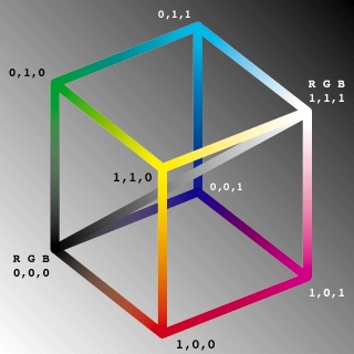
Figure 3. RGB colour cube.
The Y component contains the luminance information of the images and is in effect
a greyscale version of the image. On an RGB colour cube, this would correspond to a
line running from (0,0,0) to (1,1,1). Cb and Cr are perpendicular colour planes,
approximately green minus magenta and blue minus yellow. Note that the weightings
in the YUC equation above gives most detail to the green component and least to
the blue. This reflects the fact that the human eye is more susceptible to
variations in the colour green and less to blue.
2. Downsample CbCr components
Once the image has been converted into YCbCr colour space (if required), the Cb
and Cr components are downsampled by a factor of 2. We can do this because the
human eye gets more detail from the luminance information, than the chrominance.
This is readily apparent from step 2 of figure 2. Note how the Cr and Cb
components have much less contrast (and thus less information) than the luminance
component.
This downsampling gives an immediate 50% reduction in the size of the file - which
explains why colour images always seem smaller than greyscale images when JPEG
compressed. Downsampling ratios are expressed in the usual manner. ie. 4:1:1
means that the U and V components have been subsampled 4 times (into 4x4 pixel blocks).


Figure 4. Downsampling U & V components (of YUV) vs. R & B components (of RGB).
The human eye is more susceptible to change in luminance (grey levels)
than change in chrominance (colours). As most of the details the human eye picks
up are stored in the Y component, more error can be tolerated in the CbCr colour
components.
Figure 5. JPEG lossy compression steps 3 and 4.
3 & 4. Group Pixels into 8x8 Blocks and DCT encode
This step seems fairly obvious. Each of the three YCbCr colour planes are
encoded separately but using the same scheme. Eight by eight pixel blocks (64
pixels in total) were chosen as the size for computational simplicity. Other block
sizes have been used for other encoding schemes. For example, the Cinepak codec
used by Apple's Quicktime software uses 4x4 blocks to give very quick (but often
poorer quality) DCT encoding and decoding. Older professional video capture cards made by
Radius use 16x16 block because they can supply the extra processing power required.
If the size of the image is not a factor of 8, it is padded out to the
required size, with extra space being added on the left and bottom of the image.
When the image is decoded, these pad pixels are chopped off.
The 64 data points are DCT encoded using the equation:
The coefficient values can be converted from a floating value to an integer
at this point, but it's probably more efficient to do it after the coefficients
are scaled and the quantisation stage (step 7).
Figure 6. JPEG lossy compression steps 5 and 6.
5 & 6. Unwrap and Scale the Coefficients
The coefficients are unwrapped in the infamous 'zig-zag' pattern which just
converts the 8x8 array into a single 64 element array with the coefficients of
most significance occurring first.
These coefficients are then scaled - except for the DC component which is the
scaled average intensity value of the entire image (or YUV plane, in the case of a colour
image). The quantisation factors used in scaling the coefficients is not actually
dictated in the JPEG specification. The encoding algorithm can actually use whatever
scale factors it likes, as these are included with the final data. The JPEG standard
has a generic set of quantisation factors which are often used.
Quantisation achieves two goals:
- It allows more detail to be kept in the (more important) low frequency data
- It averages to zero, coefficient values which are close to zero
Figure 7. JPEG lossy compression steps 7 to 10.
7. Quantise and Eliminate Near Zero Coefficients
Next, coefficients which have been scaled to near zero values are actually given
zero values, in the hope that there will be many zero coefficients and therefore
compress well. This is the second lossy part of the compression
process, where we deliberately and irretrievably loose information.
The major lossy part of the JPEG process is quantisation, where each coefficient
is divided by its own scale factor. The larger this number is, the more compression will be
applied to the image data. This step is where the intended quality of the final
image can be specified. Although it is possible to calculation and encode custom
quantisation tables, in practice the default ISO JPEG tables are used most of
the time.
8 & 9. Huffman Encode Data and add Header Info
The resulting quantised integer coefficients are then Huffman encoded to squeeze
that extra bit of compression out of the image. Huffman compression is lossless
of course. Header information is added tot he data, including the quantisation
factor, the scale factors and the Huffman tables. Do a bit of formatting and
out squirts a JPEG file!
Decompressing JPEG images
The JPEG compression scheme can be described as asymmetrical, in that the method
used for compression, when reversed, is the method for decompression.
- Remove header info and quantisation factors.
- Extract data from Huffman encode bit stream.
- Scale each coefficient by the inverse 'quantisation' factors.
- Prepare the coefficients for IDCT in 8x8 blocks.
- IDCT each coefficient block.
- Put the 8x8 pixel blocks into the image buffer.
- Scale up the CbCr components.
- Convert the YCbCr components into an RGB image.
The main difference in decoding is the use of the Inverse Discrete Cosine Transform,
which is:
Progressing Encoding/decoding
There is a progressive mode available as part of the JPEG standard which, like
interlaced GIF images, allows a quick 'preview' of the image to be viewed. The
standard JPEG image data is arranged with DC components and 8x8 DCT coefficient
blocks running left to right, top to bottom through the image.
The progressive mode allows the DC
components to be sent first, followed by the DCT coefficients in a low-
frequency to high-frequency order. This enables the decoder to reproduce a low
quality version of the image quickly, before successive (higher frequency)
coefficients and received and decoded. The image data can be organised into two
or more 'strips' of DCT information, resulting in two or more possible preview
images.
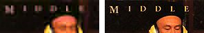
Figure 8. Two step progressive JPEG decoding.
The principle advantage of this mode is the ability to quickly view a low quality
version of the image. The Disadvantages are:
- The file size of images JPEG encoded this way are slightly increased.
- The decoder requires a buffer for all the partial (and final) DCT
coefficients.
- The decoder has to recompute and display the final image every time it
receives a new strip of DCT information.
There are some questions you can try to answer
on JPEG encoding.
How did you find this 'lecture'? Was it too hard? Too easy? Were there something in
particular you would like graphically illustrated? If you have any sensible comments,
email me and let me know.
References: